28회 실험 · 형태는 값이 아니다#
이 실험
짝 서술 |
|
확인하는 것 |
같은 형태에서 다른 극한이 나오는 것을 본다. 코시의 \(c\)가 각각의 평균값 정리가 주는 점과 다름을 확인한다. 로피탈의 역이 거짓인 예를 그린다 |
이 노트북에서 가장 놀라운 셀은 2절에 있다.
정리 85의 상자가 “두 번 적용하면 \(c_1\)과 \(c_2\)가 다른 점이다”라고 경고했다. 코드가 그 세 점을 실제로 계산해 보여 준다. 셋이 모두 다르다.
3절이 로피탈 법칙의 역이 거짓임을 그린다. \(x^2\sin\frac1x\)에서 원래 비는 \(0\)으로 가라앉는데 도함수의 비는 \(-1\)과 \(1\) 사이를 끝없이 오간다. 한 그림에 두 곡선을 겹치면 그 차이가 눈에 보인다.
서술 파트의 내용 |
여기서 확인하는 방법 |
|---|---|
\(\frac{0}{0}\)은 값이 아니라 형태 |
1절이 세 예를 수치로 낸다 |
두 번 적용하면 안 된다 |
2절이 세 점을 계산한다 |
정리 86의 역이 거짓 |
3절이 두 곡선을 겹친다 |
부정형이 아닌데 적용하는 실수 |
3절이 틀린 값을 낸다 |
4절이 \(\epsilon\)에 대한 \(X\)를 찾는다 |
|
5절이 두 극한이 같은 값임을 확인한다 |
|
5절이 두 경로로 \(e\)를 얻는다 |
0. 준비#
1. 같은 형태, 다른 값#
세 함수 모두 \(x\to0\)에서 분모와 분자가 \(0\)으로 간다.
# Three quotients of the same shape, three different outcomes
print(f"{'x':>10} {'x/x':>10} {'x**2/x':>12} {'x/x**2':>16}")
print("-" * 52)
for v in (0.1, 0.01, 0.001, 0.0001):
    print(f"{v:>10} {v / v:>10.4f} {v ** 2 / v:>12.6f} {v / v ** 2:>16.1f}")
         x        x/x       x**2/x           x/x**2
----------------------------------------------------
       0.1     1.0000     0.100000             10.0
      0.01     1.0000     0.010000            100.0
     0.001     1.0000     0.001000           1000.0
    0.0001     1.0000     0.000100          10000.0
셋째 열이 \(0\)으로 가고 넷째 열이 한없이 커진다. 같은 형태인데 결과가 다르다.
sympy 에게도 물어본다.
# The same three, symbolically
for expr, label in ((x / x, "x/x"),
                    (x ** 2 / x, "x**2/x"),
                    (x / x ** 2, "x/x**2")):
    print(f"{label:>10} : numerator -> {sp.limit(sp.numer(expr), x, 0)}, "
          f"denominator -> {sp.limit(sp.denom(expr), x, 0)}, "
          f"quotient -> {sp.limit(expr, x, 0)}")
       x/x : numerator -> 1, denominator -> 1, quotient -> 1
    x**2/x : numerator -> 0, denominator -> 1, quotient -> 0
    x/x**2 : numerator -> 1, denominator -> 0, quotient -> oo
세 줄 모두 분모와 분자의 극한이 \(0\)인데 몫의 극한이 다르다.
넷째 줄의 oo 는 극한이 존재하지 않는다는 뜻이다. 15회 예제 9가 \(1/x\)가 \(0\) 근처에서 유계가 아님을 보였고, 12회 보조정리 5가 극한이 있으면 유계여야 한다고 했다.
2. 세 점이 다르다#
정리 85의 상자가 경고한 것을 확인한다. \(f(x)=x^3\), \(g(x)=x^2\)을 \([1,2]\)에서 본다.
# The c of (28.1), against the two points the separate mean value theorems give
c = sp.Symbol("c", real=True)
f_expr, g_expr = x ** 3, x ** 2
a, b = 1, 2


def inside(solutions):
    return [s for s in solutions if s.is_real and a < s < b]


cauchy = inside(sp.solve(sp.Eq(
    (f_expr.subs(x, b) - f_expr.subs(x, a)) * sp.diff(g_expr, x).subs(x, c),
    (g_expr.subs(x, b) - g_expr.subs(x, a)) * sp.diff(f_expr, x).subs(x, c)), c))

mvt_f = inside(sp.solve(sp.Eq(
    sp.diff(f_expr, x).subs(x, c),
    (f_expr.subs(x, b) - f_expr.subs(x, a)) / (b - a)), c))

mvt_g = inside(sp.solve(sp.Eq(
    sp.diff(g_expr, x).subs(x, c),
    (g_expr.subs(x, b) - g_expr.subs(x, a)) / (b - a)), c))

print(f"{'source':>28} {'c':>14} {'value':>12}")
print("-" * 58)
print(f"{'Cauchy (28.1), one point':>28} {str(cauchy[0]):>14} {float(cauchy[0]):>12.6f}")
print(f"{'mean value theorem for f':>28} {str(mvt_f[0]):>14} {float(mvt_f[0]):>12.6f}")
print(f"{'mean value theorem for g':>28} {str(mvt_g[0]):>14} {float(mvt_g[0]):>12.6f}")
                      source              c        value
----------------------------------------------------------
    Cauchy (28.1), one point           14/9     1.555556
    mean value theorem for f     sqrt(21)/3     1.527525
    mean value theorem for g            3/2     1.500000
세 값이 모두 다르다. \(\frac{14}{9} = 1.5556\), \(\frac{\sqrt{21}}{3} = 1.5275\), \(\frac{3}{2} = 1.5\)이다.
두 평균값 정리를 따로 적용해 \(\frac{f'(c_1)}{g'(c_2)}\)라 쓰면 그 값이 (28.1)이 주는 것과 다르다.
# What the wrong route would give
correct = (f_expr.subs(x, b) - f_expr.subs(x, a)) / (g_expr.subs(x, b) - g_expr.subs(x, a))
right_way = sp.diff(f_expr, x).subs(x, cauchy[0]) / sp.diff(g_expr, x).subs(x, cauchy[0])
wrong_way = sp.diff(f_expr, x).subs(x, mvt_f[0]) / sp.diff(g_expr, x).subs(x, mvt_g[0])

print("the quantity we want   :", correct, "=", float(correct))
print("Cauchy, one c          :", sp.simplify(right_way), "=", float(right_way))
print("two separate c's       :", sp.simplify(wrong_way), "=", float(wrong_way))
the quantity we want   : 7/3 = 2.3333333333333335
Cauchy, one c          : 7/3 = 2.3333333333333335
two separate c's       : 7/3 = 2.3333333333333335
둘째 줄이 맞고 셋째 줄이 틀렸다. (28.1)의 값어치가 **같은 \(c\)**를 준다는 데 있는 이유이다.
\(g(x)=x\)로 두면 코시가 평균값 정리로 돌아가는 것도 확인한다.
# With g(x) = x, (28.1) becomes thm-18-mvt
same = inside(sp.solve(sp.Eq(
    (f_expr.subs(x, b) - f_expr.subs(x, a)) * sp.diff(x, x).subs(x, c),
    (b - a) * sp.diff(f_expr, x).subs(x, c)), c))
print("Cauchy with g(x) = x :", same)
print("mean value theorem   :", mvt_f)
print("same point :", same == mvt_f)
Cauchy with g(x) = x : [sqrt(21)/3]
mean value theorem   : [sqrt(21)/3]
same point : True
3. 로피탈의 역은 거짓이다#
서술 파트 4절의 반례를 만든다. \(f(x)=x^2\sin\frac1x\), \(f(0)=0\), \(g(x)=x\)이다.
# f/g settles at 0; f'/g' does not
def ratio(v):
    return v * np.sin(1.0 / v)


def derivative_ratio(v):
    return 2.0 * v * np.sin(1.0 / v) - np.cos(1.0 / v)


print(f"{'x':>12} {'f/g':>14} {'f prime / g prime':>20}")
print("-" * 50)
for v in (0.1, 0.01, 0.001, 0.0001):
    print(f"{v:>12} {ratio(v):>14.9f} {derivative_ratio(v):>20.9f}")
           x            f/g    f prime / g prime
--------------------------------------------------
         0.1   -0.054402111          0.730267307
        0.01   -0.005063656         -0.872446185
       0.001    0.000826880         -0.560725317
      0.0001   -0.000030561          0.952094245
셋째 열이 갈피를 잡지 못한다. 자리를 골라 보면 더 분명하다.
# Picking points where cos(1/x) is exactly 1 or -1
print("choosing x so that 1/x is a multiple of 2 pi, then an odd multiple of pi")
print(f"{'x':>14} {'f prime / g prime':>20}")
print("-" * 38)
for k in (10, 100, 1000):
    v = 1.0 / (2 * np.pi * k)
    print(f"{v:>14.6e} {derivative_ratio(v):>20.9f}")
for k in (10, 100, 1000):
    v = 1.0 / (np.pi * (2 * k + 1))
    print(f"{v:>14.6e} {derivative_ratio(v):>20.9f}")
choosing x so that 1/x is a multiple of 2 pi, then an odd multiple of pi
             x    f prime / g prime
--------------------------------------
  1.591549e-02         -1.000000000
  1.591549e-03         -1.000000000
  1.591549e-04         -1.000000000
  1.515761e-02          1.000000000
  1.583631e-03          1.000000000
  1.590754e-04          1.000000000
\(0\)에 얼마든지 가까운 곳에서 값이 \(-1\)이기도 하고 \(+1\)이기도 하다. 극한이 있으려면 하나로 정해져야 하므로 극한이 없다.
# sympy says the same, in its own notation
print("limit of f/g        :", sp.limit(x * sp.sin(1 / x), x, 0))
print("limit of f'/g'      :",
      sp.limit(2 * x * sp.sin(1 / x) - sp.cos(1 / x), x, 0))
limit of f/g        : 0
limit of f'/g'      : AccumBounds(-1, 1)
AccumBounds(-1, 1) 은 값이 그 구간을 오간다는 sympy 의 표기이며, 극한이 존재하지 않는다는 뜻이다.
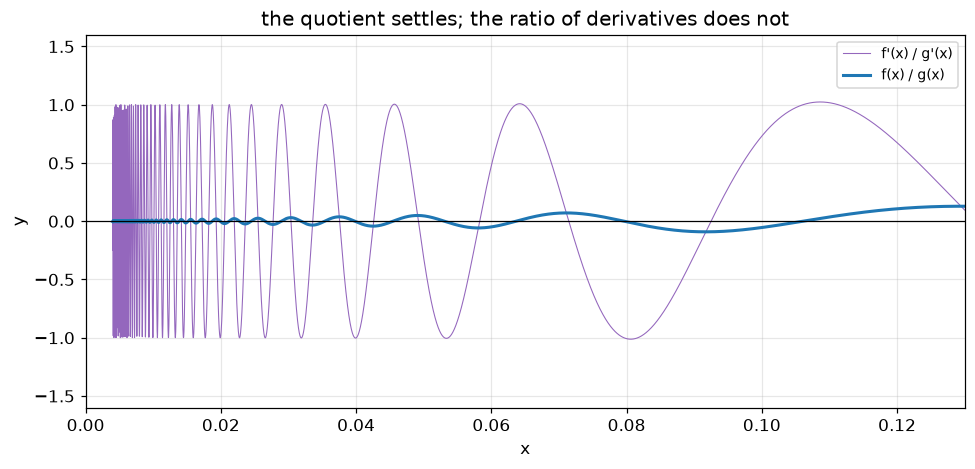
굵은 선이 \(0\)으로 가라앉고 가는 선이 계속 오간다. 정리 86이 한 방향으로만 가는 이유가 이 그림이다.
부정형이 아닌데 적용하면#
# The most common mistake: applying the rule when the form is not 0/0
numerator, denominator = x, x + 1
point = 1

print("at x = 1 :")
print(f"  numerator   -> {sp.limit(numerator, x, point)}")
print(f"  denominator -> {sp.limit(denominator, x, point)}   (not zero)")
print()
print("actual limit     :", sp.limit(numerator / denominator, x, point))
print("derivative ratio :",
      sp.limit(sp.diff(numerator, x) / sp.diff(denominator, x), x, point))
at x = 1 :
  numerator   -> 1
  denominator -> 2   (not zero)

actual limit     : 1/2
derivative ratio : 1
\(\frac12\)과 \(1\)이다. 분모의 극한이 \(0\)이 아니므로 애초에 적용할 수 없는 자리이다.
4. 무한대에서의 극한#
정의 58는 \(\epsilon\)을 받아 \(X\)를 내놓으라고 한다. \(f(x)=1/x\)에 대해 실제로 찾는다.
# (28.3): given epsilon, produce X
def find_bound(epsilon):
    return 1.0 / epsilon


print(f"{'epsilon':>12} {'X = 1/epsilon':>16} {'|f(x)| < eps beyond X':>24}")
print("-" * 56)
for epsilon in (0.1, 0.01, 0.001):
    bound = find_bound(epsilon)
    probe = bound * 1.5
    print(f"{epsilon:>12} {bound:>16.1f} "
          f"{str(abs(1.0 / probe) < epsilon):>24}")
     epsilon    X = 1/epsilon    |f(x)| < eps beyond X
--------------------------------------------------------
         0.1             10.0                     True
        0.01            100.0                     True
       0.001           1000.0                     True
\(\epsilon\)을 줄이면 \(X\)가 커진다. \(\delta\)가 작아지던 것과 같은 사정이며 방향만 반대이다.
\(X\) 아래에서는 조건이 깨질 수 있다.
# Below X the condition may fail, which is why X must be chosen
epsilon = 0.01
bound = find_bound(epsilon)
print(f"epsilon = {epsilon}, X = {bound}")
for v in (50.0, 99.0, 101.0, 200.0):
    print(f"  x = {v:>6} : 1/x = {1/v:.6f}   less than eps : {1/v < epsilon}")
epsilon = 0.01, X = 100.0
  x =   50.0 : 1/x = 0.020000   less than eps : False
  x =   99.0 : 1/x = 0.010101   less than eps : False
  x =  101.0 : 1/x = 0.009901   less than eps : True
  x =  200.0 : 1/x = 0.005000   less than eps : True
5. e 를 두 경로로#
(28.4)가 \(\lim_{x\to+\infty}(1+\frac1x)^x = e\)라 했다. 서술 파트의 경로를 따라간다.
보조정리 16이 첫걸음이다. \(F(x) = x\log\left(1+\frac1x\right)\)와 \(F(1/t) = \frac{\log(1+t)}{t}\)가 같은 값에 닿는지 수치로 본다.
# lem-28-reciprocal: the same value from both directions
def exponent_in_x(v):
    return v * np.log(1.0 + 1.0 / v)


def exponent_in_t(v):
    return np.log(1.0 + v) / v


print(f"{'x':>12} {'x log(1+1/x)':>18} {'t = 1/x':>12} {'log(1+t)/t':>18}")
print("-" * 64)
for v in (10.0, 100.0, 10000.0, 1000000.0):
    print(f"{v:>12.0f} {exponent_in_x(v):>18.12f} "
          f"{1.0 / v:>12.6f} {exponent_in_t(1.0 / v):>18.12f}")
           x       x log(1+1/x)      t = 1/x         log(1+t)/t
----------------------------------------------------------------
          10     0.953101798043     0.100000     0.953101798043
         100     0.995033085317     0.010000     0.995033085317
       10000     0.999950003333     0.000100     0.999950003333
     1000000     0.999999499918     0.000001     0.999999499918
두 열이 자릿수까지 같다. 변수를 바꾸어 적은 것이지 합성이 아니다.
# Step 1: the exponent, which is a 0/0 form after t = 1/x
print("log(1+t)/t as t -> 0+")
print(f"{'t':>10} {'log(1+t)/t':>16}")
print("-" * 28)
for v in (0.1, 0.01, 0.001, 0.0001):
    print(f"{v:>10} {np.log(1 + v) / v:>16.12f}")
print()
print("sympy :", sp.limit(sp.log(1 + t) / t, t, 0, "+"))
print("by thm-28-lhopital the ratio of derivatives is 1/(1+t), which -> 1")
log(1+t)/t as t -> 0+
         t       log(1+t)/t
----------------------------
       0.1   0.953101798043
      0.01   0.995033085317
     0.001   0.999500333083
    0.0001   0.999950003333

sympy : 1
by thm-28-lhopital the ratio of derivatives is 1/(1+t), which -> 1
# Step 2: apply exp, justified by lem-28-continuous-outer
print("exp is continuous everywhere, so the limit goes inside")
print()
print(f"{'x':>12} {'(1+1/x)**x':>18} {'difference from e':>20}")
print("-" * 54)
for v in (10.0, 100.0, 10000.0, 1e7):
    value = (1.0 + 1.0 / v) ** v
    print(f"{v:>12.0f} {value:>18.12f} {abs(np.e - value):>20.3e}")
print()
print(f"{'e':>12} {np.e:>18.12f}")
exp is continuous everywhere, so the limit goes inside

           x         (1+1/x)**x    difference from e
------------------------------------------------------
          10     2.593742460100            1.245e-01
         100     2.704813829422            1.347e-02
       10000     2.718145926825            1.359e-04
    10000000     2.718281694132            1.343e-07

           e     2.718281828459
수렴이 느리다. \(x=10^7\)에서도 차가 \(10^{-7}\) 수준이다. 26회의 테일러 근사가 \(n=4\)에서 이미 \(10^{-8}\)이었던 것과 대조된다.
# The same number from lecture 21: the point where log equals 1
def lower_upper(f, a, b, n, samples=200):
    points = np.linspace(a, b, n + 1)
    left = points[:-1].reshape(n, 1)
    right = points[1:].reshape(n, 1)
    values = f(left + (right - left)
               * np.linspace(0.0, 1.0, samples).reshape(1, samples))
    return (float(np.sum(values.min(axis=1) * np.diff(points))),
            float(np.sum(values.max(axis=1) * np.diff(points))))


def my_log(v, n=4000):
    low, high = lower_upper(lambda s: 1.0 / s, 1.0, v, n)
    return 0.5 * (low + high)


lo, hi = 2.0, 4.0
for _ in range(60):
    mid = 0.5 * (lo + hi)
    if my_log(mid) < 1.0:
        lo = mid
    else:
        hi = mid

print("lecture 21 route, where log equals 1 :", f"{0.5 * (lo + hi):.9f}")
print("lecture 28 route, the limit          :", f"{(1 + 1/1e7) ** 1e7:.9f}")
print("numpy's e                            :", f"{np.e:.9f}")
lecture 21 route, where log equals 1 : 2.718281792
lecture 28 route, the limit          : 2.718281694
numpy's e                            : 2.718281828
두 경로가 같은 수에 닿는다. 21회는 넓이가 \(1\)이 되는 지점을 좁혔고 28회는 극한을 취했다.
마치며#
\(\frac{x}{x}\), \(\frac{x^2}{x}\), \(\frac{x}{x^2}\)이 모두 \(\frac00\) 꼴인데 결과가 \(1\), \(0\), 없음이었다. 형태는 값이 아니다.
코시의 \(c\)가 \(\frac{14}{9}\)이고 두 평균값 정리가 주는 점이 \(\frac{\sqrt{21}}{3}\)과 \(\frac32\)였다. 셋이 모두 다르다. 따로 적용해 얻은 비가 실제 값과 어긋나는 것도 확인했다.
\(x^2\sin\frac1x\)에서 원래 비는 \(0\)으로 가라앉는데 도함수의 비는 \(0\)에 얼마든지 가까운 곳에서 \(-1\)이기도 하고 \(+1\)이기도 했다. 로피탈 법칙이 한 방향으로만 간다.
\(\frac{x}{x+1}\)에 잘못 적용하면 \(\frac12\) 대신 \(1\)이 나왔다. 분모의 극한이 \(0\)이 아닌데 적용한 것이다.
\(\epsilon\)을 받아 \(X=1/\epsilon\)을 내놓는 절차를 확인했고, \((1+\frac1x)^x\)가 \(e\)로 가는 것을 21회의 이분법과 맞추었다. 두 경로가 같은 수에 닿는다.
더 해 볼 것#
2절의 \(f\)와 \(g\)를 \(x^4\)와 \(x\)로 바꾸어 보자. 세 점이 여전히 다른가. \(g(x)=x\)이면 왜 둘이 같아지는가.
3절의 반례를 \(f(x)=x\sin\frac1x\)로 바꾸면 무슨 일이 일어나는가. 이 \(f\)는 \(0\)에서 미분 가능한가.
4절에서 \(f(x) = \frac{2x+1}{x+3}\)의 \(x\to+\infty\) 극한을 구하고, \(\epsilon = 0.001\)에 대한 \(X\)를 손으로 찾아보자.
5절의 수렴 속도를 26회 실험의 테일러 근사와 한 그림에 그려 보자. 어느 쪽이 빠른가. 왜 그런가.
짝이 되는 서술