18회 실험 · 한 점에서 구간으로#
이 실험
짝 서술 |
|
확인하는 것 |
평균값 정리의 \(c\)를 실제로 찾고 둘일 수 있음을 본다. 가정이 빠지면 \(c\)가 사라지는 것을 확인한다. 도함수의 부호에서 읽은 결론을 함숫값으로 검산한다 |
정리 59는 \(c\)가 있다고만 말한다. 어디인지는 말하지 않는다. 14회 중간값 정리에서 본 것과 같은 사정이다.
그런데 이번에는 사정이 조금 다르다. 중간값 정리에서는 근을 이분법으로 좁힐 수 있었지만, 여기서 \(c\)를 찾으려면 \(f'(c)\)가 평균 변화율과 같아지는 지점을 찾아야 하고 그것은 \(f'\)에 대한 또 하나의 방정식이다. 1절이 그 방정식을 풀어 \(c\)가 하나가 아닐 수 있음을 보인다.
2절이 반례를 다룬다. \(|x|\)에서 \(c\)가 없다는 것을 눈으로 확인한다. 단 한 점에서 미분 가능성이 빠진 것으로 결론이 사라진다.
3절이 이 회차의 요점이다. 정리 60은 도함수의 부호라는 점마다의 정보에서 함수가 증가한다는 구간 전체의 결론을 끌어낸다. 그 두 가지를 따로 계산해 대조한다. 도함수의 부호는 격자 위에서 확인하고 증가 여부는 함숫값의 차로 확인하며, 둘은 서로 다른 계산이다.
서술 파트의 내용 |
여기서 확인하는 방법 |
|---|---|
(18.5)의 \(c\) |
1절이 방정식을 풀어 \(c\)를 구한다 |
\(c\)가 유일하지 않다 |
1절이 \(x^3-x\)에서 두 개를 얻는다 |
\(\lvert x\rvert\) 반례 |
2절이 \(f'\)의 값이 \(\pm1\)뿐임을 보인다 |
끝점의 미분 가능성은 필요 없다 |
2절이 \(x^{1/2}\)로 \(c\)를 찾는다 |
3절이 부호와 함숫값을 따로 계산해 맞춘다 |
|
3절이 도함수가 같은 두 함수의 차를 본다 |
|
4절이 부호 변화로 극값을 판정한다 |
0. 준비#
이 회차에서 쓸 것만 불러온다. 접선과 할선을 그리므로 그 두 색을 둔다.
1. c 를 실제로 찾는다#
(18.5)은 \(f'(c)\)가 평균 변화율과 같다고 한다. 두 값을 각각 계산하고 방정식을 푼다.
# Average rate of change on the left, and the equation f'(c) = that value
t = sp.Symbol("t", real=True)


def mean_value_points(expr, a, b):
    f = sp.lambdify(t, expr, "numpy")
    slope = sp.Rational(sp.nsimplify(f(b) - f(a)), sp.nsimplify(b - a))
    solutions = sp.solve(sp.Eq(sp.diff(expr, t), slope), t)
    inside = [r for r in solutions if r.is_real and a < float(r) < b]
    return slope, inside


for expr, a, b in ((t ** 2, 1, 3), (t ** 3 - t, -2, 2)):
    slope, points = mean_value_points(expr, a, b)
    print(f"f = {str(expr):<10} on [{a},{b}]  slope = {slope}")
    print(f"    c 개수 = {len(points)}   c = {[sp.nsimplify(r) for r in points]}")
f = t**2       on [1,3]  slope = 4
    c 개수 = 1   c = [2]
f = t**3 - t   on [-2,2]  slope = 3
    c 개수 = 2   c = [-2*sqrt(3)/3, 2*sqrt(3)/3]
첫 줄에서 \(c\)가 하나이고 둘째 줄에서 둘이다. 정리는 하나 있다고만 했고 몇 개인지는 말하지 않았다.
\(x^3-x\)의 두 \(c\)가 실제로 조건을 만족하는지 되짚는다.
# Check both c values satisfy f'(c) = slope
expr = t ** 3 - t
slope, points = mean_value_points(expr, -2, 2)
derivative = sp.diff(expr, t)
for c in points:
    print(f"c = {float(c):>10.6f}   f'(c) = {sp.simplify(derivative.subs(t, c))}"
          f"   slope = {slope}")
c =  -1.154701   f'(c) = 3   slope = 3
c =   1.154701   f'(c) = 3   slope = 3
그림으로 보면 할선과 평행한 접선이 두 개이다.
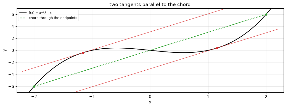
세 직선의 기울기가 모두 \(3\)이다. 할선 하나와 접선 둘이 평행하다.
2. 가정이 빠지면 c 가 사라진다#
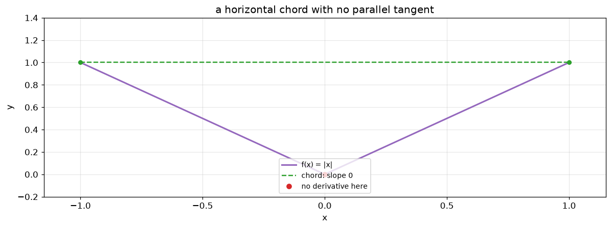
\(f(x)=|x|\)를 \([-1,1]\)에서 본다. 이 함수는 연속이지만 16회 예제 11에 의하여 \(0\)에서 미분 가능하지 않다.
# The average rate of change is 0, but f' is never 0
average = (abs(1.0) - abs(-1.0)) / (1.0 - (-1.0))
print("average rate of change on [-1,1] :", average)

grid = np.linspace(-1.0, 1.0, 21)
print(f"\n{'x':>8} {'f prime':>12}")
print("-" * 22)
for x in grid[::4]:
    if x == 0.0:
        print(f"{x:>8} {'does not exist':>12}")
    else:
        print(f"{x:>8} {(1.0 if x > 0 else -1.0):>12.1f}")
average rate of change on [-1,1] : 0.0

       x      f prime
----------------------
    -1.0         -1.0
    -0.6         -1.0
-0.19999999999999996         -1.0
0.20000000000000018          1.0
0.6000000000000001          1.0
     1.0          1.0
도함수값이 \(1\) 아니면 \(-1\)이고 \(0\)인 곳이 없다. \(x=0\)에서는 값 자체가 없다. 평균 변화율 \(0\)에 도달하는 \(c\)가 없다.
끝점에서는 없어도 된다#
반대로 끝점에서의 미분 가능성은 필요하지 않다. \(f(x)=x^{1/2}\)를 \([0,1]\)에서 보면 \(0\)에서 미분 가능하지 않은데도 정리를 쓸 수 있다.
# x**(1/2) on [0,1]: not differentiable at 0, but 0 is not in the open interval
y = sp.Symbol("y", positive=True)
root = y ** sp.Rational(1, 2)
slope = (1 - 0) / (1 - 0)
solutions = sp.solve(sp.Eq(sp.diff(root, y), slope), y)
print("f' =", sp.diff(root, y))
print("average rate of change :", slope)
print("c solving f'(c) = 1    :", solutions)
print("inside (0,1) :", [r for r in solutions if 0 < float(r) < 1])
f' = 1/(2*sqrt(y))
average rate of change : 1.0
c solving f'(c) = 1    : [0.250000000000000]
inside (0,1) : [0.250000000000000]
\(c=1/4\)이고 \((0,1)\) 안에 있다. 17회 정리 56가 \(y>0\)에서만 도함수를 주었으므로 \(0\)은 빠져 있는데, 정리 59가 요구하는 것도 열린구간뿐이라 어긋나지 않는다.
한쪽은 내부의 한 점이 빠져 무너지고 다른 쪽은 끝점이 빠져도 멀쩡하다. 가정에서 \([a,b]\)와 \((a,b)\)를 나누어 쓴 이유가 이것이다.
3. 한 점에서 구간으로#
이 절이 정리 60을 확인한다. 두 가지를 따로 계산해 맞추는 것이 요점이다.
왼쪽: 격자 위에서 \(f'\)의 부호를 본다. 점마다의 정보이다.
오른쪽: 함숫값의 차를 본다. 구간 전체의 결론이다.
정리는 왼쪽에서 오른쪽으로 가는 다리이고, 코드는 두 끝을 각각 재어 다리가 놓였는지 본다.
# Left: the sign of f' on a grid. Right: whether the values actually increase.
expr = t ** 3 - 3 * t
derivative = sp.diff(expr, t)
f = sp.lambdify(t, expr, "numpy")
df = sp.lambdify(t, derivative, "numpy")

print("f  =", expr, "    f' =", sp.factor(derivative))
print()
print(f"{'interval':>16} {'sign of f prime':>18} {'values increase':>17} "
      f"{'values decrease':>17}")
print("-" * 74)
for lo, hi in ((-3.0, -1.0), (-1.0, 1.0), (1.0, 3.0)):
    interior = np.linspace(lo, hi, 400)[1:-1]
    if (df(interior) > 0).all():
        sign = "positive"
    elif (df(interior) < 0).all():
        sign = "negative"
    else:
        sign = "mixed"
    values = f(np.linspace(lo, hi, 400))
    rising = bool(np.all(np.diff(values) > 0))
    falling = bool(np.all(np.diff(values) < 0))
    print(f"{f'[{lo:g}, {hi:g}]':>16} {sign:>18} {str(rising):>17} "
          f"{str(falling):>17}")
f  = t**3 - 3*t     f' = 3*(t - 1)*(t + 1)

        interval    sign of f prime   values increase   values decrease
--------------------------------------------------------------------------
        [-3, -1]           positive              True             False
         [-1, 1]           negative             False              True
          [1, 3]           positive              True             False
부호가 양수인 두 구간에서 함숫값이 오르고, 음수인 구간에서 내린다. 격자에서 읽은 것과 함숫값에서 읽은 것이 맞는다.
격자는 증명이 아니다
왼쪽 열은 \(f'\)을 398개 점에서만 본 것이다. 그 사이에 부호가 바뀌는 자리가 있어도 이 코드는 놓친다.
그리고 오른쪽 열도 400개 함숫값의 차를 본 것이지 모든 두 점을 본 것이 아니다. 정의 33은 구간의 임의의 두 점을 요구한다.
두 유한한 확인을 잇는 것이 정리 59이고, 그 정리는 유한 번의 계산으로 얻어지지 않는다. 코드가 하는 일은 정리가 참일 때 무엇이 보이는지를 보이는 것이다.
도함수가 같으면 차가 상수#
따름정리 9를 확인한다. 도함수가 같은 두 함수를 만들고 차를 본다.
# Two functions with the same derivative differ by a constant
first = t ** 3 - 3 * t
second = t ** 3 - 3 * t + 5

print("f' - g' =", sp.simplify(sp.diff(first, t) - sp.diff(second, t)))
print("f  - g  =", sp.simplify(first - second))

f1 = sp.lambdify(t, first, "numpy")
f2 = sp.lambdify(t, second, "numpy")
grid = np.linspace(-2.0, 2.0, 9)
differences = f1(grid) - f2(grid)
print("\ndifferences on a grid :", np.unique(np.round(differences, 12)))
f' - g' = 0
f  - g  = -5

differences on a grid : [-5.]
격자 위 아홉 점에서 차가 모두 \(-5\) 하나이다. (18.7)의 \(k\)가 그 값이다.
\(k\)가 \(0\)이라고 말할 수 없다는 것도 이 출력이 보인다. 도함수는 같은데 두 함수는 다르다.
4. 곡선 그리기#
\(f(x)=x^3-3x\)의 모양을 4절과 5절의 도구로 읽는다. 순서는 도함수의 영점 → 부호 변화 → 극값 → 이계도함수 → 볼록이다.
# The whole analysis of section 5, in the order the narrative does it
critical = sp.solve(sp.Eq(derivative, 0), t)
print("f'  =", sp.factor(derivative), "   zeros :", critical)

second_derivative = sp.diff(expr, t, 2)
print("f'' =", second_derivative, "   zeros :", sp.solve(sp.Eq(second_derivative, 0), t))

print()
print(f"{'point':>8} {'f':>8} {'sign of f prime left':>22} "
      f"{'right':>10} {'verdict':>12}")
print("-" * 66)
for c in critical:
    c = float(c)
    left = float(derivative.subs(t, c - 0.1))
    right = float(derivative.subs(t, c + 0.1))
    verdict = ("local max" if left > 0 > right
               else "local min" if left < 0 < right else "neither")
    print(f"{c:>8.1f} {float(expr.subs(t, c)):>8.1f} "
          f"{'positive' if left > 0 else 'negative':>22} "
          f"{'positive' if right > 0 else 'negative':>10} {verdict:>12}")
f'  = 3*(t - 1)*(t + 1)    zeros : [-1, 1]
f'' = 6*t    zeros : [0]

   point        f   sign of f prime left      right      verdict
------------------------------------------------------------------
    -1.0      2.0               positive   negative    local max
     1.0     -2.0               negative   positive    local min
\(x=-1\)에서 극댓값 \(2\)이고 \(x=1\)에서 극솟값 \(-2\)이다. 정리 61가 판정한 것이 이것이다.
\(f''(x)=6x\)이므로 \(x=0\)에서 볼록의 방향이 바뀐다.
# Convexity from the sign of the second derivative
for lo, hi in ((-2.0, 0.0), (0.0, 2.0)):
    interior = np.linspace(lo, hi, 200)[1:-1]
    values = np.array([float(second_derivative.subs(t, x)) for x in interior])
    shape = "convex (f'' > 0)" if (values > 0).all() else "concave (f'' < 0)"
    print(f"[{lo:g}, {hi:g}] : {shape}")
[-2, 0] : concave (f'' < 0)
[0, 2] : convex (f'' > 0)
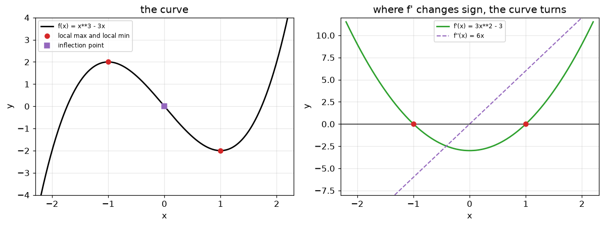
오른쪽 그림에서 \(f'\)이 축을 가로지르는 두 점이 왼쪽 그림의 두 봉우리·골짜기와 같은 \(x\)이다.
마치며#
\(x^2\)을 \([1,3]\)에서 보아 \(c=2\) 하나를 얻었고, \(x^3-x\)를 \([-2,2]\)에서 보아 \(c\)가 둘임을 확인했다. 정리는 하나 있다고만 말한다.
\(|x|\)를 \([-1,1]\)에서 보았더니 평균 변화율 \(0\)에 도달하는 \(c\)가 없었다. 도함수값이 \(\pm1\)뿐이고 \(0\)에서는 아예 없다. 반대로 \(x^{1/2}\)는 \(0\)에서 미분 가능하지 않은데도 \(c=1/4\)을 주었다. 내부의 한 점이 빠지는 것과 끝점이 빠지는 것이 다르다.
3절이 이 회차의 요점이었다. 격자 위에서 잰 \(f'\)의 부호와 함숫값의 차에서 읽은 증가·감소가 세 구간에서 모두 맞았다. 두 계산은 서로 독립이고 그것을 잇는 것이 평균값 정리이다.
도함수가 같은 두 함수의 차가 아홉 점에서 모두 \(-5\)였다. \(0\)이 아니라는 것이 따름정리 9가 상수까지만 말하는 이유이다.
더 해 볼 것#
1절의
mean_value_points에 \(f(x)=x^3\)과 \([-1,1]\)을 넣어 보자. \(c\)가 몇 개인가. 그중 \((-1,1)\) 안에 있는 것은 몇 개인가.2절의 \(|x|\)를 \([0,1]\)에서 보면 어떻게 되는가. 그 구간에서는 \(c\)가 있는가. 왜 사정이 달라지는가.
3절의 격자를 \(400\)개에서 \(5\)개로 줄여 보자. 세 구간의 판정이 그대로인가. 「격자는 증명이 아니다」 상자의 지적이 실제로 문제가 되는 함수를 하나 만들어 보자.
4절의 \(f\)를 \(x^4-2x^2\)으로 바꾸어 전체 분석을 다시 돌려 보자. 임계점이 셋인데 그중 극값이 아닌 것이 있는가. 정리 61의 부호 조건으로 판정해 보자.
짝이 되는 서술