25회 실험 · 절차가 언제나 끝난다#
이 실험
짝 서술 |
|
확인하는 것 |
나눗셈과 부분분수 분해를 손으로 한 것과 sympy 가 한 것을 맞춘다. 계수를 두 방법으로 정한다. 절댓값을 빠뜨리면 어디서 무너지는지 본다 |
이 노트북의 주제는 절차이다.
22회와 23회의 기법은 통할지 미리 알 수 없었다. 유리함수는 다르다. 서술 파트 5절의 흐름도가 유한 번에 끝나며, 그 각 단계를 코드로 옮길 수 있다.
3절이 이 노트북에서 가장 값어치 있는 자리이다. sympy 의 apart 가 부분분수 분해를 한 줄에 해 주는데, 그 한 줄이 무엇을 하는지를 계수 비교로 직접 재현한다. 두 결과가 맞으면 서술 파트 3절의 절차가 옳다는 뜻이다.
4절이 절댓값을 다룬다. sympy 는 \(\int\frac{dx}{x-2}\)에 \(\log(x-2)\)를 돌려주는데 절댓값이 없다. 그것이 어디서 문제가 되는지 본다.
서술 파트의 내용 |
여기서 확인하는 방법 |
|---|---|
1절이 나눗셈을 하고 \(\deg R < \deg D\)를 확인한다 |
|
2절 인수분해 |
2절이 실근의 유무를 본다 |
(25.3)의 계수 결정 |
3절이 두 방법을 나란히 놓는다 |
중복 인수 |
3절이 \(\frac{x}{(x-1)^2}\)을 분해한다 |
(25.4)의 절댓값 |
4절이 빠뜨렸을 때를 본다 |
5절 구체적 값 |
5절이 상합·하합으로 좁힌다 |
0. 준비#
# The integral of definition 7, used to check the closed-form answers
def lower_upper(f, a, b, n, samples=200):
    points = np.linspace(a, b, n + 1)
    left = points[:-1].reshape(n, 1)
    right = points[1:].reshape(n, 1)
    values = f(left + (right - left)
               * np.linspace(0.0, 1.0, samples).reshape(1, samples))
    return (float(np.sum(values.min(axis=1) * np.diff(points))),
            float(np.sum(values.max(axis=1) * np.diff(points))))
1. 나눗셈#
정리 79이 \(P = QD + R\)과 \(\deg R < \deg D\)를 준다. 두 조건을 각각 확인한다.
# thm-25-division: divide, then check both conclusions
numerator = x ** 4 + 2 * x ** 2 - 1
denominator = x ** 2 - 1

quotient, remainder = sp.div(numerator, denominator, x)
print("P =", numerator)
print("D =", denominator)
print("Q =", quotient)
print("R =", remainder)
print()
print("Q*D + R - P    =", sp.simplify(sp.expand(quotient * denominator + remainder - numerator)))
print("deg R =", sp.degree(remainder, x), " < deg D =", sp.degree(denominator, x))
P = x**4 + 2*x**2 - 1
D = x**2 - 1
Q = x**2 + 3
R = 2

Q*D + R - P    = 0
deg R = 0  < deg D = 2
두 조건이 모두 성립한다.
증명이 절차였다는 것도 확인해 둔다. 최고차 항을 지우는 한 단계를 손으로 적어 본다.
# One step of the proof: kill the leading term and see the degree drop
leading_p = sp.LC(sp.Poly(numerator, x))
leading_d = sp.LC(sp.Poly(denominator, x))
gap = sp.degree(numerator, x) - sp.degree(denominator, x)

reduced = sp.expand(numerator - (leading_p / leading_d) * x ** gap * denominator)
print("after one step :", reduced)
print("degree dropped from", sp.degree(numerator, x), "to", sp.degree(reduced, x))
after one step : 3*x**2 - 1
degree dropped from 4 to 2
차수가 \(4\)에서 \(2\)로 줄었다. 한 단계마다 줄어들므로 유한 번에 끝난다.
2. 인수분해#
서술 파트 2절이 실계수 다항식은 일차식과 실근이 없는 이차식의 곱이라고 했다.
# Factoring over the reals: quadratics without real roots stay whole
for expr in (x ** 3 - x, x ** 3 + x, x ** 4 - 1, x ** 2 + 1, x ** 2 - 2):
    print(f"{str(expr):>10}  ->  {sp.factor(expr)}")
  x**3 - x  ->  x*(x - 1)*(x + 1)
  x**3 + x  ->  x*(x**2 + 1)
  x**4 - 1  ->  (x - 1)*(x + 1)*(x**2 + 1)
  x**2 + 1  ->  x**2 + 1
  x**2 - 2  ->  x**2 - 2
\(x^2+1\)이 쪼개지지 않았다. 실근이 없기 때문이다.
# Why x**2 + 1 stays whole: no real root
for expr in (x ** 2 + 1, x ** 2 - 1):
    real_roots = [r for r in sp.solve(sp.Eq(expr, 0), x) if r.is_real]
    print(f"{str(expr):>10} : real roots = {real_roots}")
  x**2 + 1 : real roots = []
  x**2 - 1 : real roots = [-1, 1]
\(x^2-2\)는 쪼개졌다. \(\sqrt2\)가 무리수이지만 실수이므로 근이 있다. 17회 정의 35가 그 수를 만들었다.
쪼개지는지는 계수가 유리수인지와 무관하다. 실근이 있느냐만 본다.
3. 부분분수 분해#
sympy 에게 시켜 본다.
# What sympy does in one line
print("1/(x**3 - x)  =", sp.apart(1 / (x ** 3 - x), x))
1/(x**3 - x) = 1/(2*(x + 1)) + 1/(2*(x - 1)) - 1/x
그 한 줄이 무엇을 한 것인지 재현한다. 서술 파트 3절의 두 방법을 각각 코드로 옮긴다.
# Method 1: match coefficients, as (25.3) does
A, B, C = sp.symbols("A B C")
identity = A * (x - 1) * (x + 1) + B * x * (x + 1) + C * x * (x - 1) - 1

equations = [sp.Eq(coefficient, 0)
             for coefficient in sp.Poly(sp.expand(identity), x).all_coeffs()]
print("the three equations :")
for equation in equations:
    print("   ", equation)
print()
print("solution :", sp.solve(equations, [A, B, C], dict=True))
the three equations :
    Eq(A + B + C, 0)
    Eq(B - C, 0)
    Eq(-A - 1, 0)

solution : [{A: -1, B: 1/2, C: 1/2}]
# Method 2: plug in the roots of the denominator
right_side = A * (x - 1) * (x + 1) + B * x * (x + 1) + C * x * (x - 1)
for point, unknown, name in ((0, A, "A"), (1, B, "B"), (-1, C, "C")):
    value = sp.solve(sp.Eq(right_side.subs(x, point), 1), unknown)
    print(f"  x = {point:>2}  ->  {name} = {value[0]}")
  x =  0  ->  A = -1
  x =  1  ->  B = 1/2
  x = -1  ->  C = 1/2
두 방법이 같은 답을 준다. 값을 넣는 쪽이 짧다. 분모의 근을 넣으면 세 항 가운데 둘이 사라지기 때문이다.
그런데 그 방법이 언제나 통하지는 않는다.
# With a repeated factor, plugging in roots is not enough
print("x/(x-1)**2  =", sp.apart(x / (x - 1) ** 2, x))
print()
print("check by combining :",
      sp.simplify(sp.together(1 / (x - 1) + 1 / (x - 1) ** 2) - x / (x - 1) ** 2))
x/(x-1)**2  = 1/(x - 1) + (x - 1)**(-2)

check by combining : 0
\(x=1\)을 넣으면 두 항이 동시에 무한이 되므로 값을 넣는 방법이 쓸 수 없다. 계수 비교로 가야 한다.
서술 파트의 흔한 오해 상자가 지적한 것이 이것이다. \((x-1)^2\)에 항을 하나만 두면 분해가 되지 않는다.
# One term is not enough for a repeated factor
single = sp.symbols("A1")
attempt = sp.solve(sp.Eq(single, x), single)
print("trying A/(x-1)**2 alone means solving A = x, which has no constant solution")
print("sympy's answer needs two terms :", sp.apart(x / (x - 1) ** 2, x))
trying A/(x-1)**2 alone means solving A = x, which has no constant solution
sympy's answer needs two terms : 1/(x - 1) + (x - 1)**(-2)
이차 인수가 있는 경우도 본다.
# A quadratic factor gets a numerator of the form Bx + C
print("1/(x**3 + x)        =", sp.apart(1 / (x ** 3 + x), x))
print("(x+2)/((x-1)(x**2+4)) =", sp.apart((x + 2) / ((x - 1) * (x ** 2 + 4)), x))
1/(x**3 + x)        = -x/(x**2 + 1) + 1/x
(x+2)/((x-1)(x**2+4)) = -(3*x - 2)/(5*(x**2 + 4)) + 3/(5*(x - 1))
이차 인수의 분자에 \(x\)가 남는다. (25.2)의 둘째 형태가 \(\frac{Bx+C}{\cdots}\)인 이유이다.
4. 절댓값을 빠뜨리면#
(25.4)가 \(\int\frac{dx}{x-a}=\log|x-a|+C\)라 했다. sympy 에게 물어본다.
# sympy drops the absolute value
print("sympy :", sp.integrate(1 / (x - 2), x))
sympy : log(x - 2)
절댓값이 없다. sympy 는 복소수 로그를 쓰는 규약이라 그렇게 적는데, 이 책의 \(\log\)는 21회 정의 46가 \(x>0\)에서만 정의했다.
\(x<2\)인 쪽에서 무슨 일이 일어나는지 본다.
# On x < 2 the version without the absolute value has no value
for v in (3.0, 2.5, 1.5, 1.0):
    inside = v - 2.0
    with_abs = np.log(abs(inside))
    without = np.log(inside) if inside > 0 else None
    print(f"x = {v:<5} x-2 = {inside:>5}   log|x-2| = {with_abs:>9.6f}   "
          f"log(x-2) = {'undefined' if without is None else f'{without:9.6f}'}")
x = 3.0   x-2 =   1.0   log|x-2| =  0.000000   log(x-2) =  0.000000
x = 2.5   x-2 =   0.5   log|x-2| = -0.693147   log(x-2) = -0.693147
x = 1.5   x-2 =  -0.5   log|x-2| = -0.693147   log(x-2) = undefined
x = 1.0   x-2 =  -1.0   log|x-2| =  0.000000   log(x-2) = undefined
아래 두 줄에서 절댓값 없는 쪽이 값을 갖지 않는다.
미분해서 확인하면 두 쪽 모두 \(\frac{1}{x-2}\)이 나온다. 21회 따름정리 12가 그것이었다.
# Both sides of x = 2, checked numerically
def derivative_of_log_abs(v, step=1e-6):
    return (np.log(abs(v + step - 2)) - np.log(abs(v - step - 2))) / (2 * step)


print(f"{'x':>7} {'d/dx log|x-2|':>18} {'1/(x-2)':>14}")
print("-" * 42)
for v in (3.0, 2.5, 1.5, 1.0):
    print(f"{v:>7} {derivative_of_log_abs(v):>18.9f} {1.0 / (v - 2.0):>14.9f}")
      x      d/dx log|x-2|        1/(x-2)
------------------------------------------
    3.0        1.000000000    1.000000000
    2.5        2.000000000    2.000000000
    1.5       -2.000000000   -2.000000000
    1.0       -1.000000000   -1.000000000
\(x=2\)의 양쪽에서 모두 맞는다. 그런데 22회의 상자가 적은 대로 \(+C\)는 한 구간 안에서만 상수 하나이다. \(x=2\)가 정의역을 두 조각으로 끊는다.
5. 절차를 끝까지#
\(\int_2^3\frac{dx}{x^2-1}\)을 서술 파트 5절의 절차대로 계산하고, 7회의 정의로 검산한다.
# The whole procedure on one integral
integrand = 1 / (x ** 2 - 1)
print("step 1  deg P < deg D, no division needed")
print("step 2  factor :", sp.factor(x ** 2 - 1))
print("step 3  apart  :", sp.apart(integrand, x))
print()
exact = sp.integrate(integrand, (x, 2, 3))
print("step 4  value  :", sp.simplify(exact), "=", float(exact))
print("         (1/2) log(3/2) =", float(sp.log(sp.Rational(3, 2)) / 2))
step 1  deg P < deg D, no division needed
step 2  factor : (x - 1)*(x + 1)
step 3  apart  : -1/(2*(x + 1)) + 1/(2*(x - 1))
step 4  value  : -log(2)/2 + log(3)/2 = 0.2027325540540822
         (1/2) log(3/2) = 0.2027325540540822
# Check against the definition of the integral
low, high = lower_upper(lambda t: 1.0 / (t ** 2 - 1), 2.0, 3.0, 20000)
print(f"lower sum  {low:.9f}")
print(f"upper sum  {high:.9f}")
print(f"exact      {float(exact):.9f}")
print(f"traps it   {low <= float(exact) <= high}")
lower sum  0.202727346
upper sum  0.202737762
exact      0.202732554
traps it   True
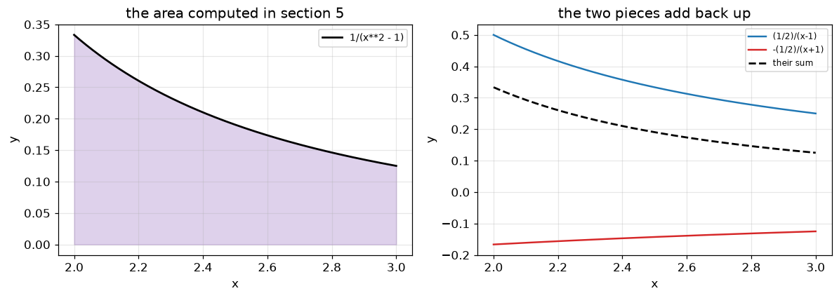
오른쪽 그림에서 두 조각의 합이 점선과 겹친다. 분해가 옳다는 것을 눈으로 확인하는 것이며, 계수 비교가 보장하는 것이 그것이다.
마치며#
나눗셈을 하고 \(\deg R < \deg D\)를 확인했고, 한 단계에서 차수가 \(4\)에서 \(2\)로 떨어지는 것을 보았다. 매번 줄어들므로 절차가 끝난다.
\(x^2+1\)이 쪼개지지 않고 \(x^2-2\)는 쪼개졌다. 실근이 있느냐만 본다.
apart 한 줄이 하는 일을 두 방법으로 재현했고 같은 답이 나왔다. 값을 넣는 방법이 짧지만 중복 인수에서는 쓸 수 없다. \(x/(x-1)^2\)에서 그것을 확인했다.
sympy 가 \(\int\frac{dx}{x-2}\)에 절댓값 없는 답을 돌려주었다. \(x<2\)에서 그 식이 값을 갖지 않는다. 21회 따름정리 12가 그 자리를 메운다.
\(\int_2^3\frac{dx}{x^2-1}\)을 절차대로 계산해 \(\frac12\log\frac32 = 0.2027\ldots\)을 얻었고, 이만 조각의 상합과 하합이 그 값을 가두었다.
더 해 볼 것#
1절의 나눗셈을 \(P=x^5-1\), \(D=x^2+1\)로 바꾸어 보자. 몫과 나머지가 무엇인가. 한 단계씩 손으로 따라가면 몇 번 만에 끝나는가.
3절의
apart에 \(\frac{1}{(x-1)^3}\)을 넣어 보자. 항이 몇 개 나오는가. \(\frac{x^2}{(x-1)^3}\)은 어떠한가.4절에서 \(\int_1^3\frac{dx}{x-2}\)를 계산하려 하면 무슨 일이 일어나는가. 그 구간에 \(x=2\)가 있는 것이 왜 문제인가. 22회의 \(\int_0^\pi\tan x\,dx\)와 같은 사정인가.
5절의 적분 구간을 \([0,\frac12]\)로 바꾸어 보자. 절댓값이 어떻게 작용하는가. 답의 부호는 어떻게 되는가.
짝이 되는 서술