13회 실험 · 판정 도구와 그 한계#
이 실험
짝 서술 |
|
확인하는 것 |
12회까지의 판정 기준을 하나의 절차로 묶고, 그 절차가 틀린 답을 내는 경우를 확인한다 |
서술 파트 2절에서 적분 가능성 판정 절차를 만들었다. 이 노트북에서는 그 절차를 코드로 옮긴다. 흐름도의 각 갈래가 함수 하나의 분기가 되고, 판정의 근거가 된 정리 이름이 반환값에 들어간다.
그다음 이 도구가 틀린 답을 내는 경우를 본다. 도구는 표본으로 함숫값을 보는데, 디리클레 함수는 표본으로 볼 수 없는 함수이다. 도구는 “단조이므로 적분 가능”이라고 답하고, 그 답은 틀렸다.
마지막으로 진동의 대비를 표로 확인한다. 서술 파트의 (13.1)과 (13.2)가 갈리는 지점이다.
서술 파트의 내용 |
여기서 확인하는 방법 |
|---|---|
2절 판정 절차 |
도구가 흐름도와 같은 순서로 묻고 답한다 |
단조인지 조각이 몇 개인지를 먼저 센다 |
|
정리 25의 \(n\)등분 형태 |
\(U_n - L_n < \epsilon\)이 되는 최초의 \(n\)을 찾는다 |
도구가 틀린 답을 내는 것을 본다 |
|
\(n\)을 키우며 \(U_n - L_n\)을 나란히 본다 |
0. 준비#
이 회차에서 쓸 것만 불러온다. 보라색은 반례를 가리킨다.
1. 판정 절차를 도구로 만든다#
먼저 상합과 하합이 필요하다. 7회 정의 11과 정의 13을 이 파일 안에서 다시 정의한다.
각 부분구간의 최댓값과 최솟값은 표본으로 근사한다. 이 근사가 뒤에서 도구를 무너뜨리는 자리이므로 셀 주석에 그 사실을 적어 둔다.
# The max / min on each subinterval are approximated by samples.
# This approximation is where the tool will later give a wrong answer.
def partition(a, b, n):
    """Return the n + 1 division points of the equal partition of [a, b]."""
    return np.linspace(a, b, n + 1)


def step_integral(points, heights):
    """Integral of the step function that takes heights[k] on the k-th subinterval."""
    return float(np.sum(np.asarray(heights) * np.diff(points)))


def lower_upper_sums(f, a, b, n, samples=200):
    """Return (lower, upper) for the equal partition of [a, b] into n pieces."""
    points = partition(a, b, n)
    left = points[:-1].reshape(n, 1)
    right = points[1:].reshape(n, 1)
    weights = np.linspace(0.0, 1.0, samples).reshape(1, samples)
    values = f(left + (right - left) * weights)
    return (step_integral(points, values.min(axis=1)),
            step_integral(points, values.max(axis=1)))
흐름도의 세 번째와 네 번째 갈래를 위해 단조인지, 조각이 몇 개인지를 세는 함수가 필요하다. 표본에서 차분의 부호가 몇 번 바뀌는지 보면 된다.
# How many monotone pieces? One means monotonic (def-10-monotone)
def monotone_pieces(f, a, b, samples=2001):
    """Count sign changes of the sampled difference, plus one."""
    xs = np.linspace(a, b, samples)
    diffs = np.diff(f(xs))
    signs = np.sign(np.where(np.abs(diffs) < 1e-12, 0.0, diffs))
    nonzero = signs[signs != 0]
    if nonzero.size == 0:
        return 1
    return 1 + int(np.count_nonzero(np.diff(nonzero) != 0))


print("x**2 on [0,1]    :", monotone_pieces(lambda x: x ** 2, 0.0, 1.0))
print("x**2-3x on [0,3] :", monotone_pieces(lambda x: x ** 2 - 3 * x, 0.0, 3.0))
print("|x-1| on [0,2]   :", monotone_pieces(lambda x: np.abs(x - 1.0), 0.0, 2.0))
x**2 on [0,1]    : 1
x**2-3x on [0,3] : 2
|x-1| on [0,2]   : 2
이제 흐름도를 그대로 옮긴다. 묻는 순서가 서술 파트 2절의 순서와 같고, 각 답에 근거가 된 정리의 라벨이 붙는다.
# The flow chart of section 2, in the same order
def diagnose(f, a, b, eps=1e-3, n_max=2 ** 14):
    """Follow the decision procedure and report which theorem settles it."""
    values = f(np.linspace(a, b, 2001))
    if not np.all(np.isfinite(values)):
        return {"verdict": "cannot decide",
                "reason": "not bounded on the samples; def-7-lower-upper does not apply"}

    pieces = monotone_pieces(f, a, b)
    if pieces == 1:
        ends = abs(float(f(np.array([b]))[0]) - float(f(np.array([a]))[0]))
        return {"verdict": "integrable", "reason": "thm-10-monotone",
                "pieces": 1, "gap_times_n": (b - a) * ends}
    if pieces <= 8:
        return {"verdict": "integrable", "reason": "thm-10-piecewise", "pieces": pieces}

    n = 1
    while n <= n_max:
        lower, upper = lower_upper_sums(f, a, b, n)
        if upper - lower < eps:
            return {"verdict": "integrable", "reason": "thm-8-riemann (n-fold form)",
                    "n": n, "gap": upper - lower}
        n *= 2
    return {"verdict": "undecided", "reason": "the n-fold form is only sufficient"}


cases = (
    ("x**2       on [0,1]", lambda x: x ** 2, 0.0, 1.0),
    ("x**2 - 3x  on [0,3]", lambda x: x ** 2 - 3 * x, 0.0, 3.0),
    ("|x - 1|    on [0,2]", lambda x: np.abs(x - 1.0), 0.0, 2.0),
    ("sin(20x)   on [0,1]", lambda x: np.sin(20 * x), 0.0, 1.0),
)
for name, fn, a, b in cases:
    report = diagnose(fn, a, b)
    print(f"{name} -> {report['verdict']:>10}  by {report['reason']}")
x**2       on [0,1] -> integrable  by thm-10-monotone
x**2 - 3x  on [0,3] -> integrable  by thm-10-piecewise
|x - 1|    on [0,2] -> integrable  by thm-10-piecewise
sin(20x)   on [0,1] -> integrable  by thm-10-piecewise
네 함수가 각각 다른 갈래에서 판정된다. \(x^2\)은 단조이므로 정리 31에서 끝나고, \(x^2-3x\)와 \(|x-1|\)은 조각이 둘이므로 정리 32로 간다.
\(\sin(20x)\)는 조각이 일곱이다. 서술 파트 2절이 지적한 대로 조각의 개수를 미리 알아야 정리 32를 쓸 수 있는데, 여기서는 표본을 세어 알아낸 것이다.
2. 도구가 틀린 답을 내는 곳#
디리클레 함수를 넣어 본다. 8회 실험에서 보았듯이 부동소수는 모두 유리수이므로 표본추출은 이 함수를 상수함수 \(1\)로 본다.
# Every float is rational, so the sampled Dirichlet function looks constant
def dirichlet_sampled(x):
    """1 on rationals, 0 on irrationals. Every float is rational, so this is 1."""
    return np.ones_like(np.asarray(x, dtype=float))


report = diagnose(dirichlet_sampled, 0.0, 1.0)
print("the tool says :", report)
print()
print("but ex-10-dirichlet proves the lower integral is 0 and the upper is 1")
print("so the function is NOT integrable")
the tool says : {'verdict': 'integrable', 'reason': 'thm-10-monotone', 'pieces': 1, 'gap_times_n': 0.0}

but ex-10-dirichlet proves the lower integral is 0 and the upper is 1
so the function is NOT integrable
도구가 “단조이므로 적분 가능”이라고 답한다. 그 답은 틀렸다.
무엇이 잘못되었는지 짚어 둔다. 도구의 어느 단계도 논리적으로 틀리지 않았다. 표본에서 차분이 전부 \(0\)이므로 조각이 하나이고, 조각이 하나이면 정리 31이 적분 가능성을 준다. 틀린 것은 입력이다. 표본이 본 함수와 실제 함수가 다르다.
10회 보조정리 4에 의하여 모든 부분구간에 유리수와 무리수가 함께 있으므로 실제로는 각 부분구간에서 최댓값이 \(1\)이고 최솟값이 \(0\)이다. 손으로 따진 값을 넣어 비교한다.
# What the sums really are, computed from lem-10-dense instead of from samples
def dirichlet_by_hand(a, b, n):
    """Every subinterval holds a rational and an irrational, so inf = 0 and sup = 1."""
    points = partition(a, b, n)
    return step_integral(points, np.zeros(n)), step_integral(points, np.ones(n))


header = f"{'n':>6} {'sampled U - L':>16} {'true U - L':>14}"
print(header)
print("-" * len(header))
for n in (1, 10, 100, 1000):
    lo_s, hi_s = lower_upper_sums(dirichlet_sampled, 0.0, 1.0, n)
    lo_h, hi_h = dirichlet_by_hand(0.0, 1.0, n)
    print(f"{n:>6} {hi_s - lo_s:>16.6f} {hi_h - lo_h:>14.6f}")
     n    sampled U - L     true U - L
--------------------------------------
     1         0.000000       1.000000
    10         0.000000       1.000000
   100         0.000000       1.000000
  1000         0.000000       1.000000
두 열이 정반대의 답을 준다. 왼쪽은 모든 \(n\)에서 \(0\)이고 오른쪽은 모든 \(n\)에서 \(1\)이다.
이 표가 도구의 경계를 보여 준다. 판정 절차는 함숫값을 볼 수 있는 함수에만 쓸 수 있고, 볼 수 없는 함수에서는 정의로 돌아가야 한다.
3. 진동의 대비#
서술 파트 2절이 세 경우를 진동 \(\omega_k\) 하나로 읽었다. (13.1)과 (13.2)의 차이를 수치로 확인한다.
증가함수에서는 진동의 합이 망원합이 되어 \(f(b)-f(a)\)로 고정되고, 디리클레 함수에서는 \(n\)이 된다.
# (13.1) : the sum is fixed.  (13.2) : the sum grows with n
def oscillation_sum(f, a, b, n):
    """Sum of the oscillations of a monotonic f, from the endpoint differences."""
    return float(np.sum(np.abs(np.diff(f(partition(a, b, n))))))


header = (f"{'n':>6} {'sum for x**2':>14} {'U-L for x**2':>14}"
          f" {'sum for Dirichlet':>19} {'U-L for Dirichlet':>19}")
print(header)
print("-" * len(header))
for n in (10, 100, 1000):
    monotone_total = oscillation_sum(lambda x: x ** 2, 0.0, 1.0, n)
    print(f"{n:>6} {monotone_total:>14.6f} {monotone_total / n:>14.6f}"
          f" {float(n):>19.6f} {1.0:>19.6f}")
     n   sum for x**2   U-L for x**2   sum for Dirichlet   U-L for Dirichlet
----------------------------------------------------------------------------
    10       1.000000       0.100000           10.000000            1.000000
   100       1.000000       0.010000          100.000000            1.000000
  1000       1.000000       0.001000         1000.000000            1.000000
\(x^2\)의 진동 합은 \(n\)이 무엇이든 \(1\)이다. (13.1)이 말하는 \(f(1)-f(0)=1\)이며, \(1/n\)을 곱하면 줄어든다.
디리클레 함수의 진동 합은 \(n\)이다. (13.2)가 말하는 대로이며, \(1/n\)을 곱하면 \(1\)이 되어 \(n\)과 무관하게 남는다.
그림으로 보면 차이가 분명하다.
# The gap against n, on a log scale
sizes = np.array([2 ** k for k in range(1, 12)])
gaps_monotone = np.array([1.0 / n for n in sizes])
gaps_dirichlet = np.ones_like(gaps_monotone)

fig, ax = plt.subplots()
ax.loglog(sizes, gaps_monotone, color=C_FUNC, marker="o", markersize=4,
          linewidth=1.6, label="x**2 : gap = 1/n")
ax.loglog(sizes, gaps_dirichlet, color=C_CEX, marker="s", markersize=4,
          linewidth=1.6, label="Dirichlet : gap = 1")
ax.set_xlabel("number of subintervals n")
ax.set_ylabel("U_n - L_n")
ax.set_title("the gap shrinks for a monotonic function and does not for Dirichlet")
ax.legend()
fig.tight_layout()
plt.show()
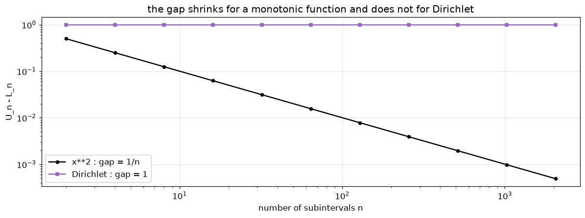
로그 눈금에서 한쪽은 기울기 \(-1\)인 직선이고 다른 쪽은 수평선이다. 적분 가능성은 이 그림에서 선이 내려가는지 아닌지의 문제이다.
마치며#
서술 파트 2절의 판정 절차를 도구로 옮겼다. 흐름도의 순서를 그대로 따르며, 각 답에 근거가 된 정리의 라벨이 붙는다. 네 함수가 각각 다른 갈래에서 판정되었다.
그다음 도구가 틀린 답을 내는 경우를 보았다. 디리클레 함수에서 도구는 “단조이므로 적분 가능”이라고 답하는데, 10회 예제 5은 적분 불가능함을 증명하였다. 도구의 논리가 틀린 것이 아니라 표본이 본 함수가 실제 함수와 다르다.
진동의 합을 나란히 놓으면 두 경우가 갈린다. 증가함수에서는 \(n\)과 무관한 상수이고 디리클레 함수에서는 \(n\)에 비례한다. 로그 눈금에서 한쪽은 내려가고 다른 쪽은 수평이다.
더 해 볼 것#
monotone_pieces의samples를 \(2001\)에서 \(21\)로 줄여 보자. \(\sin(20x)\)의 조각 수가 어떻게 달라지는가. 표본이 성기면 진동을 놓친다는 것이 도구의 또 다른 한계이다.diagnose에 \(f(x) = 1/x\)를 \([0,1]\)에서 넣어 보자. 첫 단계에서 무엇이 걸리는가. “적분 불가능하다”와 “적분을 정의할 수 없다”가 어떻게 다른지 반환값의 문구로 확인해 보자.3절의 그림에 \(x^3\)을 \([0,2]\)에서 더해 보자. 10회 (10.5)에 의하여 기울기가 \(-1\)인 직선이어야 하는데, 세로 위치는 \(x^2\)의 선과 어떻게 다른가.
짝이 되는 서술