21회 실험 · 넓이가 함수가 된다#
이 실험
짝 서술 |
|
확인하는 것 |
정의 (21.1)만으로 \(\log\)를 직접 만든다. 그 함수를 미분해 \(1/x\)가 나오는지 본다. \(e\)와 \(2^{\sqrt2}\)를 손으로 구한다 |
이 노트북은 np.log를 쓰지 않고 시작한다.
정의 46이 \(\log x = \int_1^x \frac{dt}{t}\)라고 했으므로, 19회 실험에서 만든 상합·하합 절차에 \(1/t\)를 넣으면 그것이 곧 \(\log\)이다. 라이브러리 함수는 답을 맞춰 보는 데만 쓴다.
2절이 요점이다. 그렇게 만든 함수를 차분몫에 넣으면 \(1/x\)가 나온다. 정리 70가 주장하는 것이며, 19회 실험 3절에서 \(x^2\)에 대해 한 일과 같은 구조인데 이번에는 결과가 새 함수이다.
4절에서 \(\log c = 1\)인 \(c\)를 이분법으로 찾는다. 그 수가 \(e\)이다. 원의 둘레 없이 \(\pi\)를 구한 20회 실험과 같은 방식으로, 거듭제곱 없이 \(e\)를 구한다.
서술 파트의 내용 |
여기서 확인하는 방법 |
|---|---|
1절이 상합·하합으로 \(\log\)를 만든다 |
|
\(x<1\)에서 부호가 바뀐다 |
1절이 정의 41를 코드로 넣는다 |
\(\log 2 \approx 0.693\) |
1절이 \(n\)을 키우며 좁힌다 |
2절이 차분몫과 \(1/x\)를 대조한다 |
|
3절이 세 쌍에서 확인한다 |
|
4절이 이분법으로 \(e\)를 찾는다 |
|
5절이 17회 정의와 21회 정의를 맞춘다 |
0. 준비#
1. 정의만으로 로그를 만든다#
19회 실험에서 쓴 절차를 그대로 가져온다. 분할을 만들고 각 부분구간의 최솟값과 최댓값으로 계단함수를 만들어 넓이를 더한다.
# The integral of definition 7, with the orientation convention of definition 19.1
def lower_upper(f, a, b, n, samples=200):
    points = np.linspace(a, b, n + 1)
    left = points[:-1].reshape(n, 1)
    right = points[1:].reshape(n, 1)
    weights = np.linspace(0.0, 1.0, samples).reshape(1, samples)
    values = f(left + (right - left) * weights)
    widths = np.diff(points)
    return (float(np.sum(values.min(axis=1) * widths)),
            float(np.sum(values.max(axis=1) * widths)))


def integral_by_definition(f, a, b, n=4000):
    if a == b:
        return 0.0
    if b < a:
        return -integral_by_definition(f, b, a, n)
    low, high = lower_upper(f, a, b, n)
    return 0.5 * (low + high)
이제 정의 46을 그대로 옮긴다. 한 줄이다.
# Definition 21.1, verbatim
reciprocal = lambda t: 1.0 / t


def my_log(x):
    return integral_by_definition(reciprocal, 1.0, x)
값을 확인한다. np.log는 여기서 처음이자 답을 맞춰 보는 데만 쓴다.
# Our log against the library's, which we use only as a check
print(f"{'x':>10} {'my_log(x)':>16} {'np.log(x)':>16} {'difference':>13}")
print("-" * 58)
for x in (0.25, 0.5, 1.0, 2.0, 10.0):
    print(f"{x:>10} {my_log(x):>16.9f} {np.log(x):>16.9f} "
          f"{abs(my_log(x) - np.log(x)):>13.2e}")
         x        my_log(x)        np.log(x)    difference
----------------------------------------------------------
      0.25     -1.386294405     -1.386294361      4.39e-08
       0.5     -0.693147184     -0.693147181      3.91e-09
       1.0      0.000000000      0.000000000      0.00e+00
       2.0      0.693147184      0.693147181      3.91e-09
      10.0      2.302585511      2.302585093      4.18e-07
\(x<1\)인 두 줄이 음수이다. 정의 41가 integral_by_definition의 if b < a 분기로 들어가 있다. 19회에서 세운 약속이 없으면 이 두 줄을 계산할 수 없다.
\(\log 1 = 0\)인 것은 같은 함수의 if a == b 분기이다.
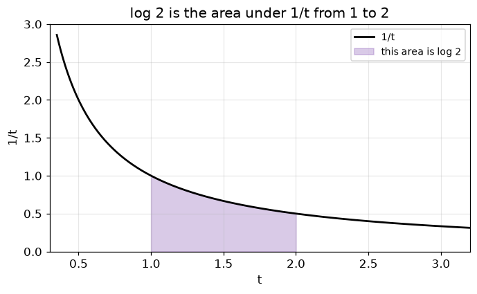
log 2 를 좁힌다#
서술 파트 7절이 \(\log 2 \approx 0.693\)이라 했다. 상합과 하합으로 실제로 좁혀 본다.
# Trapping log 2 between a lower and an upper sum, as lecture 7 would
print(f"{'n':>8} {'lower':>15} {'upper':>15} {'width':>12}")
print("-" * 54)
for n in (4, 10, 100, 1000, 10000):
    low, high = lower_upper(reciprocal, 1.0, 2.0, n)
    print(f"{n:>8} {low:>15.9f} {high:>15.9f} {high - low:>12.2e}")
       n           lower           upper        width
------------------------------------------------------
       4     0.634523810     0.759523810     1.25e-01
      10     0.668771403     0.718771403     5.00e-02
     100     0.690653430     0.695653430     5.00e-03
    1000     0.692897243     0.693397243     5.00e-04
   10000     0.693122181     0.693172181     5.00e-05
폭이 \(n\)에 반비례해 줄어든다. \(n=10000\)에서 \([0.693122,\ 0.693172]\)까지 좁혀졌다.
7회는 이 값을 닫힌 형태로 적을 수 없었다. \(\sum \frac1k\)에 공식이 없기 때문이다. 좁히는 것은 그때도 할 수 있었고, 달라진 것은 그 값에 이름이 생겼다는 것이다.
2. 만든 함수를 미분한다#
이 절이 정리 70를 확인한다. my_log는 넓이를 더해 만든 함수이고, 그것을 차분몫에 넣는다.
# The function built from areas, fed into the difference quotient
def difference_quotient(f, p, step=1e-4):
    return (f(p + step) - f(p - step)) / (2 * step)


print(f"{'p':>8} {'quotient of my_log':>21} {'1/p':>14} {'difference':>13}")
print("-" * 60)
for p in (0.5, 1.0, 2.0, 5.0):
    q = difference_quotient(my_log, p)
    print(f"{p:>8} {q:>21.9f} {1.0 / p:>14.9f} {abs(q - 1.0 / p):>13.2e}")
       p    quotient of my_log            1/p    difference
------------------------------------------------------------
     0.5           2.000000063    2.000000000      6.31e-08
     1.0           1.000000003    1.000000000      3.33e-09
     2.0           0.500000010    0.500000000      9.53e-09
     5.0           0.200000041    0.200000000      4.14e-08
네 줄 모두 맞는다.
방향이 19회와 반대라는 점이 요점이다. 19회는 도함수를 아는 함수의 적분을 구했다. 여기서는 적분으로 정의한 함수의 도함수를 얻는다. 따름정리 10가 그 통로이다.
\(1/x>0\)이므로 \(\log\)가 순증가해야 한다. 확인한다.
# Strictly increasing: every consecutive pair rises
xs = np.linspace(0.2, 8.0, 60)
values = np.array([my_log(v) for v in xs])
print("all increases positive :", bool(np.all(np.diff(values) > 0)))
print("smallest increase      :", f"{np.diff(values).min():.3e}")
all increases positive : True
smallest increase      : 1.666e-02
3. 곱셈 법칙#
정리 71를 세 쌍에서 확인한다.
# log(ab) against log a + log b
print(f"{'a':>6} {'b':>6} {'log(ab)':>16} {'log a + log b':>16} {'difference':>13}")
print("-" * 62)
for a, b in ((2.0, 3.0), (0.5, 8.0), (1.5, 1.5)):
    left = my_log(a * b)
    right = my_log(a) + my_log(b)
    print(f"{a:>6} {b:>6} {left:>16.9f} {right:>16.9f} {abs(left - right):>13.2e}")
     a      b          log(ab)    log a + log b    difference
--------------------------------------------------------------
   2.0    3.0      1.791759596      1.791759492      1.04e-07
   0.5    8.0      1.386294405      1.386294608      2.03e-07
   1.5    1.5      0.810930223      0.810930218      5.08e-09
둘째 줄이 특히 그렇다. \(\log 0.5\)가 음수이고 \(\log 8\)이 양수인데 합이 \(\log 4\)와 맞는다.
따름정리 11의 세 식도 본다.
# The three consequences of the product rule
a, b, n = 3.0, 5.0, 4
print(f"log(1/a)      = {my_log(1 / a):>12.9f}   -log a  = {-my_log(a):>12.9f}")
print(f"log(a/b)      = {my_log(a / b):>12.9f}   diff    = "
      f"{my_log(a) - my_log(b):>12.9f}")
print(f"log(a**n)     = {my_log(a ** n):>12.9f}   n log a = {n * my_log(a):>12.9f}")
log(1/a)      = -1.098612307   -log a  = -1.098612307
log(a/b)      = -0.510825625   diff    = -0.510825685
log(a**n)     =  4.394482482   n log a =  4.394449229
4. e 를 찾는다#
정의 48는 \(\log e = 1\)인 수가 \(e\)라고 했다. 그 수를 이분법으로 찾는다.
정리 72가 그런 수의 존재를 주고, 순증가가 유일성을 준다. 이분법이 옳게 도는 근거가 그 둘이다.
# Definition 21.5: e is where log equals 1. Bisection, since log is increasing.
def bisect(f, lo, hi, rounds=60):
    for _ in range(rounds):
        mid = 0.5 * (lo + hi)
        if f(mid) < 0.0:
            lo = mid
        else:
            hi = mid
    return 0.5 * (lo + hi)


print("log 2 =", f"{my_log(2.0):.9f}", " (less than 1)")
print("log 4 =", f"{my_log(4.0):.9f}", " (greater than 1)")

e_found = bisect(lambda v: my_log(v) - 1.0, 2.0, 4.0)
print()
print(f"e by bisection : {e_found:.12f}")
print(f"np.e           : {np.e:.12f}")
print(f"difference     : {abs(e_found - np.e):.2e}")
log 2 = 0.693147184  (less than 1)
log 4 = 1.386294405  (greater than 1)
e by bisection : 2.718281792316
np.e           : 2.718281828459
difference     : 3.61e-08
서술 파트가 \(\log 2 < 1 < 2\log 2\)이면 \(2<e<4\)라고 했다. 위 두 줄이 그것을 확인한다.
\(e\)를 거듭제곱의 극한으로 정의하지 않았다. 쓴 것은 넓이가 \(1\)이 되는 지점을 좁힌 것뿐이다.
5. 무리수 지수#
정의 49가 \(a^x = \exp(x\log a)\)라 했다. 1절에서 물었던 \(2^{\sqrt2}\)를 구한다.
# Definition 21.7 applied to the question of section 1
root_two = np.sqrt(2.0)
exponent = root_two * my_log(2.0)

print(f"sqrt 2        = {root_two:.12f}")
print(f"log 2         = {my_log(2.0):.12f}")
print(f"their product = {exponent:.12f}")
print()
print(f"exp of it     = {np.exp(exponent):.12f}")
print(f"2 ** sqrt 2   = {2.0 ** root_two:.12f}")
sqrt 2        = 1.414213562373
log 2         = 0.693147184466
their product = 0.980258148993

exp of it     = 2.665144157413
2 ** sqrt 2   = 2.665144142690
두 값이 같다. 오른쪽 줄은 numpy가 내부에서 하는 계산이고 왼쪽은 우리의 정의이다.
17회의 정의와 어긋나지 않는가#
정리 74가 유리수에서 두 정의가 같다고 했다. 확인한다.
# Definition 17.6 (root then power) against definition 21.7 (exp of a product)
base = 5.0
print(f"{'m/n':>8} {'lecture 17':>20} {'lecture 21':>20} {'difference':>13}")
print("-" * 66)
for m, n in ((1, 2), (2, 3), (3, 1), (5, 4)):
    by_seventeen = (base ** (1.0 / n)) ** m
    by_twentyone = np.exp((m / n) * my_log(base))
    print(f"{f'{m}/{n}':>8} {by_seventeen:>20.12f} {by_twentyone:>20.12f} "
          f"{abs(by_seventeen - by_twentyone):>13.2e}")
     m/n           lecture 17           lecture 21    difference
------------------------------------------------------------------
     1/2       2.236067977500       2.236068066943      8.94e-08
     2/3       2.924017738213       2.924017894160      1.56e-07
     3/1     125.000000000000     125.000030000000      3.00e-05
     5/4       7.476743906106       7.476744653780      7.48e-07
네 줄 모두 맞는다. 왼쪽은 \(n\)제곱근을 취한 뒤 \(m\)제곱한 것이고 오른쪽은 \(\exp\)와 \(\log\)만 쓴 것이다. 두 경로가 겹치지 않는데 값이 같다.
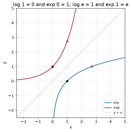
동그란 점이 \((1,0)\)과 \((0,1)\)이고 네모난 점이 \((e,1)\)과 \((1,e)\)이다. 두 곡선이 \(y=x\)에 대하여 서로의 거울상이다.
마치며#
np.log를 쓰지 않고 정의 46만으로 \(\log\)를 만들었다. 상합과 하합을 평균한 것이며, \(x<1\)에서 음수가 나오는 것은 정의 41가 코드의 if b < a 분기로 들어가 있기 때문이다.
\(\log 2\)를 \(n=10000\)에서 \([0.693122,\ 0.693172]\)까지 좁혔다. 7회도 이만큼은 할 수 있었다. 달라진 것은 그 값에 이름이 생겼다는 것이다.
그 함수를 차분몫에 넣었더니 네 점 모두에서 \(1/p\)가 나왔다. 19회 실험은 도함수를 아는 함수의 적분을 구했고, 여기서는 적분으로 만든 함수의 도함수를 얻었다. 방향이 반대이다.
\(\log\)가 \(1\)이 되는 지점을 이분법으로 좁혀 \(2.71828179\)를 얻었다. np.e와 \(10^{-8}\) 안에서 같다. 거듭제곱의 극한을 쓰지 않았다.
\(2^{\sqrt2}\)를 \(\exp(\sqrt2\log 2)\)로 계산해 \(2.665144142690\)을 얻었고, 유리수 지수에서는 17회의 정의와 21회의 정의가 열두 자리까지 맞았다.
더 해 볼 것#
1절의
integral_by_definition에서n을 \(4000\)에서 \(200\)으로 줄이고 2절의 차분몫 표를 다시 뽑아 보자. 차이 열이 얼마나 커지는가.step을 함께 줄이면 나아지는가.1절에서 \(\log\)의 정의역을 \(x \le 0\)으로 넓히려 하면 무슨 일이 일어나는가.
my_log(-1.0)을 불러 보고, 그 결과가 서술 파트의 흔한 오해 상자와 어떻게 이어지는지 적어 보자.3절의 곱셈 법칙을 \(a=b=\sqrt2\)에서 확인해 보자. \(\log 2 = 2\log\sqrt2\)인가. 그것이 정리 74와 어떻게 이어지는가.
4절의 이분법을 \(\log c = 2\)인 \(c\)에 대해 돌려 보자. 그 값이 \(e^2\)인가. \(\log c = -1\)이면 어떤 구간에서 찾아야 하는가.
짝이 되는 서술