24회 실험 · 표를 검산한다#
이 실험
짝 서술 |
|
확인하는 것 |
대조표의 열 줄을 하나씩 미분해 되돌린다. 계산 절차를 실제로 돌아가는 코드로 만든다. 사슬의 두 화살표에 반례를 세운다 |
정리편의 실험은 새 계산을 하지 않는다. 지금까지 얻은 것이 정말 맞는지 한꺼번에 검산한다.
1절이 서술 파트 1절의 대조표를 그대로 코드로 옮긴다. 각 줄의 원시함수를 미분해 피적분함수가 나오는지 본다. 열 줄이 한 번에 검사된다.
2절이 이 노트북의 요점이다. 서술 파트 2절의 계산 절차는 글로 적힌 흐름도인데, 그것을 실제로 돌아가는 함수로 만든다. 피적분함수를 넣으면 어느 기법을 쓸지 골라 준다. 그렇게 만들어 보면 흐름도에 적히지 않은 판단이 드러난다.
4절은 서술 파트 5절의 실수 표를 재현한다. 틀린 답을 실제로 출력한다.
서술 파트의 내용 |
여기서 확인하는 방법 |
|---|---|
1절 대조표 |
1절이 열 줄을 미분해 되돌린다 |
함수 목록 |
1절이 도함수를 나란히 출력한다 |
2절 계산 절차 |
2절이 분류기를 만들어 돌린다 |
4절의 사슬 |
3절이 두 화살표에 반례를 세운다 |
5절 실수 표 |
4절이 틀린 값을 실제로 낸다 |
0. 준비#
1. 대조표를 검산한다#
서술 파트 1절의 표에서 오른쪽 열은 왼쪽 열을 다시 쓴 것이라 했다. 미분해서 되돌아오면 그 말이 맞다.
# Every row of the table: differentiate the primitive, compare with the integrand
rows = [
    ("x**4", x ** 4, x ** 5 / 5, x, "thm-16-power"),
    ("x**(3/2)", xp ** sp.Rational(3, 2),
     sp.Rational(2, 5) * xp ** sp.Rational(5, 2), xp, "thm-17-rational-power"),
    ("sin x", sp.sin(x), -sp.cos(x), x, "thm-20-derivative"),
    ("cos x", sp.cos(x), sp.sin(x), x, "thm-20-derivative"),
    ("1/x", 1 / xp, sp.log(xp), xp, "thm-21-log-deriv"),
    ("exp x", sp.exp(x), sp.exp(x), x, "thm-21-exp-deriv"),
    ("1/(1+x**2)", 1 / (1 + x ** 2), sp.atan(x), x, "thm-23-inverse-deriv"),
    ("1/sqrt(1-x**2)", 1 / sp.sqrt(1 - x ** 2), sp.asin(x), x,
     "thm-23-inverse-deriv"),
]

print(f"{'integrand':>16} {'primitive':>26} {'back':>6}  from")
print("-" * 76)
for label, integrand, primitive, var, source in rows:
    back = sp.simplify(sp.diff(primitive, var) - integrand) == 0
    print(f"{label:>16} {str(primitive):>26} {str(back):>6}  {source}")
       integrand                  primitive   back  from
----------------------------------------------------------------------------
            x**4                     x**5/5   True  thm-16-power
        x**(3/2)              2*xp**(5/2)/5   True  thm-17-rational-power
           sin x                    -cos(x)   True  thm-20-derivative
           cos x                     sin(x)   True  thm-20-derivative
             1/x                    log(xp)   True  thm-21-log-deriv
           exp x                     exp(x)   True  thm-21-exp-deriv
      1/(1+x**2)                    atan(x)   True  thm-23-inverse-deriv
  1/sqrt(1-x**2)                    asin(x)   True  thm-23-inverse-deriv
여덟 줄 모두 되돌아온다. 각 줄의 마지막 칸이 그 원시함수를 준 정리이다.
곱과 합성에 대응하는 두 줄은 함수가 아니라 기법이므로 따로 확인한다.
# The two techniques, each checked against the differentiation rule it came from
f, g = x ** 2, sp.sin(x)
parts_left = sp.integrate(f * sp.diff(g, x), (x, 0, 1))
parts_right = ((f * g).subs(x, 1) - (f * g).subs(x, 0)
               - sp.integrate(sp.diff(f, x) * g, (x, 0, 1)))
print("integration by parts, two sides equal :",
      sp.simplify(parts_left - parts_right) == 0)

u = sp.Symbol("u", real=True)
inner = x ** 3 + 1
sub_left = sp.integrate(sp.sin(inner) * sp.diff(inner, x), (x, 0, 1))
sub_right = sp.integrate(sp.sin(u), (u, inner.subs(x, 0), inner.subs(x, 1)))
print("substitution, two sides equal        :",
      sp.simplify(sp.N(sub_left - sub_right)) == 0)
integration by parts, two sides equal : True
substitution, two sides equal : True
2. 절차를 코드로 만든다#
서술 파트 2절의 흐름도를 실제로 돌아가는 함수로 옮긴다. 옮겨 보면 글에 적히지 않은 판단이 드러난다.
# The flow chart of section 2, as a function that classifies an integrand
def classify(expr, var):
    """Return which technique the chart of section 2 reaches first."""
    basic = (var, sp.sin(var), sp.cos(var), sp.exp(var), 1 / var)
    if any(sp.simplify(expr - candidate) == 0 for candidate in basic):
        return "basic: use the primitive directly"
    if expr.is_polynomial(var):
        return "basic: power rule term by term"

    has_root = any(isinstance(piece, sp.Pow) and piece.exp.is_Rational
                   and piece.exp.q == 2 for piece in expr.atoms(sp.Pow))
    if has_root:
        return "trigonometric substitution"

    if expr.is_rational_function(var):
        return "rational: partial fractions (next part)"

    if isinstance(expr, sp.Mul) and len(expr.args) >= 2:
        return "product: integration by parts"

    return "none of the above: may have no elementary primitive"
몇 가지를 넣어 본다.
# Run the chart on the integrands this part has met
tests = [
    x ** 3 + 2 * x,
    sp.sin(x),
    1 / (1 + x ** 2),
    sp.sqrt(1 - x ** 2),
    x * sp.cos(x),
    sp.exp(-x ** 2),
]
for expr in tests:
    print(f"{str(expr):>18}  ->  {classify(expr, x)}")
x**3 + 2*x -> basic: power rule term by term
            sin(x)  ->  basic: use the primitive directly
      1/(x**2 + 1)  ->  rational: partial fractions (next part)
    sqrt(1 - x**2)  ->  trigonometric substitution
          x*cos(x)  ->  product: integration by parts
exp(-x**2) -> none of the above: may have no elementary primitive
흐름도가 판단을 대신하지 않는다
위 함수는 서술 파트의 흐름도를 그대로 옮겼는데, 옮기면서 결정해야 했던 것이 여럿이다.
\(\frac{1}{1+x^2}\)은 유리함수이면서 동시에 (23.5)의 기본 공식이다. 흐름도의 어느 가지에 먼저 걸리는가. 위 코드는 기본 함수 검사를 먼저 하지 않아 유리함수로 분류했는데, 그러면 부분분수로 가서 돌아가게 된다.
\(x\cos x\)는 곱이지만 \(\sin x \cdot \frac{1}{x}\)도 곱이다. 앞의 것은 부분적분으로 풀리고 뒤의 것은 초등적 원시함수가 없다. “곱인가”라는 물음만으로는 갈라지지 않는다.
흐름도의 각 가지에 “확인한다”는 줄이 붙어 있는 이유가 이것이다. 절차는 무엇을 먼저 시도할지를 말할 뿐이고, 시도가 이득인지는 해 보아야 안다.
3. 사슬의 두 화살표#
서술 파트 4절이 미분 가능 \(\Rightarrow\) 연속 \(\Rightarrow\) 적분 가능이라 했고 역이 둘 다 거짓이라 했다. 두 반례를 만든다.
# First arrow: |x| is continuous at 0 but not differentiable there
step = 1e-8
right = (abs(0.0 + step) - 0.0) / step
left = (abs(0.0 - step) - 0.0) / (-step)
print("|x| at 0")
print(f"  right difference quotient : {right:+.1f}")
print(f"  left  difference quotient : {left:+.1f}")
print(f"  values agree              : {right == left}")
print()
values = [abs(v) for v in (-1e-6, -1e-9, 0.0, 1e-9, 1e-6)]
print(f"  but the values approach f(0) = 0 : {max(values):.1e}")
|x| at 0
  right difference quotient : +1.0
  left  difference quotient : -1.0
  values agree              : False

  but the values approach f(0) = 0 : 1.0e-06
# Second arrow: a step function is integrable but not continuous
def lower_upper(f, a, b, n, samples=200):
    points = np.linspace(a, b, n + 1)
    left_edge = points[:-1].reshape(n, 1)
    right_edge = points[1:].reshape(n, 1)
    values = f(left_edge + (right_edge - left_edge)
               * np.linspace(0.0, 1.0, samples).reshape(1, samples))
    return (float(np.sum(values.min(axis=1) * np.diff(points))),
            float(np.sum(values.max(axis=1) * np.diff(points))))


jump = lambda t: np.where(t < 0.5, 0.0, 1.0)
print(f"{'n':>8} {'lower':>12} {'upper':>12} {'width':>11}")
print("-" * 46)
for n in (10, 100, 1000, 10000):
    low, high = lower_upper(jump, 0.0, 1.0, n)
    print(f"{n:>8} {low:>12.6f} {high:>12.6f} {high - low:>11.2e}")
print()
print("the two sums close on 0.5, so the step function is integrable")
print("yet it jumps at x = 0.5, so it is not continuous there")
       n        lower        upper       width
----------------------------------------------
      10     0.500000     0.600000    1.00e-01
     100     0.500000     0.510000    1.00e-02
    1000     0.500000     0.501000    1.00e-03
   10000     0.500000     0.500100    1.00e-04

the two sums close on 0.5, so the step function is integrable
yet it jumps at x = 0.5, so it is not continuous there
두 화살표 모두 한 방향으로만 간다.
\((0,1)\)에서 \(1/x\)가 셋째 반례이다. 연속인데 적분 가능하지 않다.
# On an open interval, continuity is not enough: 1/x is unbounded
print(f"{'x':>12} {'1/x':>14}")
print("-" * 28)
for v in (1e-2, 1e-4, 1e-8):
    print(f"{v:>12} {1 / v:>14.1f}")
print()
print("no bound M works, so def-7-integral does not apply")
           x            1/x
----------------------------
        0.01          100.0
      0.0001        10000.0
       1e-08    100000000.0

no bound M works, so def-7-integral does not apply
7회 정의 15이 유계를 요구하므로 이 함수에는 상적분도 하적분도 정의되지 않는다. 사슬이 닫힌구간에서의 이야기인 이유가 여기 있다.
4. 실수를 재현한다#
서술 파트 5절의 표에서 계산 실수 셋을 실제로 저질러 본다.
# Mistake 1: forgetting to change the limits in a substitution
u = sp.Symbol("u", real=True)
inner = 1 + x ** 2

direct = sp.integrate(sp.expand(2 * x * (1 + x ** 2)), (x, 0, 1))
correct = sp.integrate(u, (u, inner.subs(x, 0), inner.subs(x, 1)))
mistaken = sp.integrate(u, (u, 0, 1))

print(f"correct  : {correct}")
print(f"mistaken : {mistaken}")
print(f"check by expanding : {direct}")
correct  : 3/2
mistaken : 1/2
check by expanding : 3/2
# Mistake 2: splitting an integral across a product
both = sp.integrate(x * sp.sin(x), (x, 0, sp.pi))
apart = sp.integrate(x, (x, 0, sp.pi)) * sp.integrate(sp.sin(x), (x, 0, sp.pi))
print(f"integral of x sin x on [0, pi] : {both}   = {float(both):.6f}")
print(f"product of the two integrals   : {apart}   = {float(apart):.6f}")
print(f"equal : {sp.simplify(both - apart) == 0}")
integral of x sin x on [0, pi] : pi   = 3.141593
product of the two integrals   : pi**2   = 9.869604
equal : False
# Mistake 3: using arcsin(sin x) = x outside the restricted interval
for v in (0.4, np.pi, 4.0):
    print(f"x = {v:>9.6f}   arcsin(sin x) = {np.arcsin(np.sin(v)):+.9f}"
          f"   equal : {abs(np.arcsin(np.sin(v)) - v) < 1e-12}")
x =  0.400000   arcsin(sin x) = +0.400000000   equal : True
x =  3.141593   arcsin(sin x) = +0.000000000   equal : False
x =  4.000000   arcsin(sin x) = -0.858407346   equal : False
세 실수 모두 오류를 내지 않고 답을 준다. 그 답이 틀릴 뿐이다.
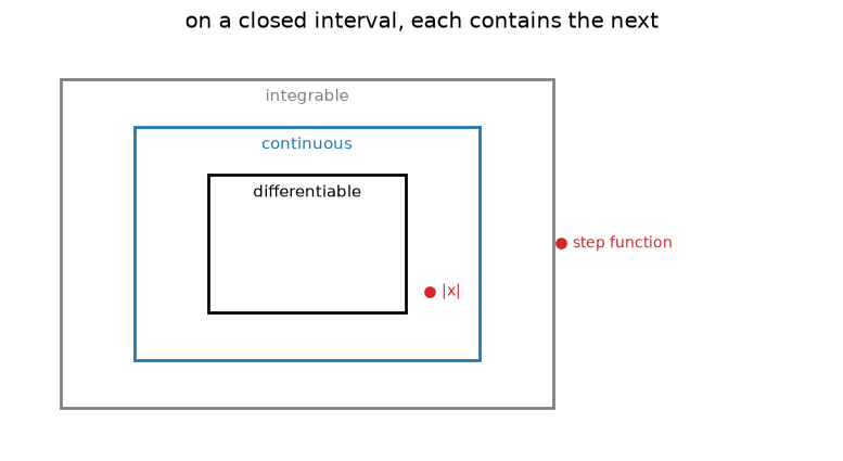
두 붉은 점이 반례이다. 계단함수는 바깥 상자에만 있고 \(|x|\)는 가운데 상자까지만 있다.
마치며#
대조표의 여덟 줄을 미분해 되돌렸고 모두 맞았다. 각 줄의 원시함수를 준 정리가 마지막 칸에 있다. 부분적분과 치환적분도 각각 양변을 따로 계산해 확인했다.
계산 절차를 함수로 옮겨 보았더니 글에 적히지 않은 판단이 드러났다. \(\frac{1}{1+x^2}\)이 기본 공식이면서 동시에 유리함수이고, “곱인가”라는 물음만으로는 \(x\cos x\)와 \(\sin x \cdot \frac1x\)를 가르지 못한다.
사슬의 두 화살표에 반례를 세웠다. \(|x|\)는 연속인데 미분 가능하지 않고, 계단함수는 적분 가능한데 연속이 아니다. \((0,1)\)의 \(1/x\)는 연속인데 유계가 아니라 적분 가능하지 않다.
실수 셋을 재현했다. 셋 다 오류를 내지 않고 틀린 답을 준다.
서술 파트의 내용 |
이 노트북의 코드 |
|---|---|
1절 대조표 |
1절 |
부분적분·치환의 출처 |
1절 |
2절 계산 절차 |
2절 |
흐름도가 판단을 대신하지 않는다 |
2절 |
4절 사슬의 첫 화살표 |
3절 \(\lvert x\rvert\) 의 좌우 차분몫 |
4절 사슬의 둘째 화살표 |
3절 계단함수의 상합·하합 |
닫힌구간이어야 한다 |
3절 \(1/x\) 가 유계가 아닌 표 |
5절 실수 표 |
4절 세 셀 |
더 해 볼 것#
2절의
classify에 기본 함수 검사를 유리함수 검사보다 먼저 오도록 고쳐 보자. \(\frac{1}{1+x^2}\)의 분류가 달라지는가. 어느 순서가 나은가.2절의
classify에 \(\frac{\log x}{x}\)를 넣어 보자. 무엇으로 분류되는가. 실제로는 어느 기법으로 풀리는가.3절의 계단함수에서 뛰는 자리를 \(x=1/3\)으로 옮기면 상합과 하합의 차가 달라지는가. \(n\)이 \(3\)의 배수일 때와 아닐 때를 비교해 보자.
1절의 표에 \(\tan\) 과 \(\sec\) 을 더해 보자. 원시함수를 적을 수 있는가. 22회와 23회의 어느 상자가 필요한가.
짝이 되는 서술