
테마
16회 · 베이즈의 귀환 · 노트
9 정리와 역사 노트
9.1 한 장 요약
| 정리 | 내용 | 조건 |
|---|---|---|
| 켤레 사전분포 (1.2) | 베타–이항, 감마–Poisson, 정규–정규: 사후평균은 정밀도 가중평균 | — |
| Laplace 근사 (1.4) | 사후분포 | 정칙, 꼭대기 하나 |
| Bayes 추정량 (2.1) | 제곱손실 → 사후평균, 절대손실 → 사후중앙값 | — |
| 허용성·minimax (2.3) | 유일한 Bayes는 허용적, 위험이 상수인 Bayes는 minimax | Bayes 위험 유한 |
| Jeffreys (2.6) | 는 모수화에 불변 | 단조 변환 |
| Bayes 인수 (3.2, 3.4) | 사후 오즈 = 사전 오즈 , | 점 귀무가설 |
| MH·Gibbs (4.5, 4.7) | 상세 균형 → 정상분포, Gibbs는 받아들임 1의 MH | 불필요 |
| Gibbs의 자기상관 (4.8) | 상관 이면 | 이변량 정규 |
| James–Stein (5.2) | 위험 | |
| 경험적 Bayes (5.4) | , 대가는 | 정규 사전분포 |
| ridge·lasso (8.1, 8.2) | 정규 사전분포의 사후평균, Laplace 사전분포의 MAP | — |
| ULA의 치우침 (8.4) | 정상분산 | 정규 목표 |
| Tweedie (8.5) | 정규 잡음 |
모수에 분포를 주면 추론은 조건부분포 하나를 계산하는 일이 된다. 그 대가는 사전분포라는 선택이고, 보상은 하나의 원리로 추정(2절), 검정(3절), 예측(연습 1.4)을 다룰 수 있다는 것이다. 계산은 MCMC가 해결했다. 그러나 이 회차의 가장 놀라운 결과는 사전분포를 믿지 않는 사람에게도 해당한다. Stein의 정리는 빈도주의의 위험으로 표현되고 증명되었다. 그런데 그 처방은 Bayes였다. 같은 종류의 양을 여럿 추정할 때는 서로에게서 빌려 와야 한다.
9.2 Stigler의 명명 법칙
이름과 발견
Bayes 정리: Bayes의 논문에는 오늘의 공식이 없다. 일반형은 Laplace(1774)의 것이다. Stigler(1983)는 반쯤 진지하게 맹인 수학자 Nicholas Saunderson이 먼저 알았을 가능성을 제기했다.
Metropolis 알고리즘: Marshall Rosenbluth의 회고(2003)에 따르면 방법을 만들고 계산한 것은 주로 Rosenbluth 부부와 Teller 부부였고, Metropolis는 컴퓨터를 맡았다. Hastings(1970)의 일반화는 오랫동안 통계학에서 주목받지 못했다.
Gibbs 표집: Geman 형제(1984)가 목표분포인 Gibbs 분포의 이름을 붙였다. 물리학자 J. W. Gibbs(1839–1903)는 표집과 관계가 없다.
James–Stein: 허용적이지 않음은 Stein(1956) 혼자 보였다. James는 명시적인 추정량을 쓴 1961년 논문의 공저자다.
Tweedie의 공식: 처음 출판한 것은 Robbins(1956)였다. Efron(2011)이 이 이름으로 다시 유행시켰다.
9.3 7 Pillars 지도 — 완성
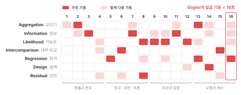
Stigler(2016)는 회귀의 장에 다변량 분석, 베이즈 추론, 인과 추론을 함께 넣었다. Galton의 2단 quincunx(5회)는 사전분포와 가능도로 사후분포를 만드는 장치였고, Stein의 축소는 Galton의 회귀였다. 그래서 이번 회차의 기둥은 Regression이다. 사후분포가 가능도에 비례한다는 점에서 Likelihood, Jeffreys 사전분포가 Fisher 정보에서 나온다는 점에서 Information, 18명의 타율을 함께 써서 각자를 더 잘 추정한다는 점에서 Aggregation도 함께 칠한다. 그림 9.1는 16회 전체의 지도다. 일곱 기둥이 모두 칠해졌다.
9.4 과정을 마치며
이 과정은 1654년 Pascal과 Fermat가 나눈 판돈에서 시작했다. 그 뒤 370년의 흐름을 정리하면 세 가지 질문이 남는다.
확률은 무엇에 대한 것인가. 1회의 공리는 답하지 않았다. 4회의 당구대와 이번 회차에서 확률은 모르는 것에 대한 믿음이었고, 8회와 12회에서는 반복되는 절차의 빈도였다. 두 해석은 대부분의 큰 표본에서 같은 숫자를 낸다(Bernstein–von Mises, 2절의 Jeffreys 구간). 갈라지는 곳은 점 귀무가설(3절)과 모수가 많은 문제(5절)다.
자료를 어떻게 줄이는가. 평균(3회), 충분통계량(11회), 최소제곱(13회), 순위(15회), 사후분포(16회)는 모두 자료를 줄이는 방법이다. 각각이 어떤 가정 아래에서 정보를 잃지 않는지가 이 과정의 정리들이 말한 것이다.
모형이 틀리면 무엇이 남는가. 6회의 검정의 로버스트성, 10회의 EM의 국소해, 15회의 붕괴점, 이번 회차의 비정칙 사후분포는 모두 정리의 조건이 깨질 때의 이야기였다. 정리를 아는 것은 그 조건을 아는 것이다.
마지막 회차의 마지막 절은 신경망의 생성모형이 1956년의 두 논문 위에 서 있다는 것으로 끝났다. 오늘의 방법은 대부분 이 과정에서 본 오래된 아이디어의 새 조합이다. 이름과 맥락은 바뀌어도 정리는 남는다.
참고문헌
Bayes, T. An essay towards solving a problem in the doctrine of chances. Phil. Trans. 53 (1763), 370–418. · Laplace, P. S. Mémoire sur la probabilité des causes par les événements. (1774). · Théorie analytique des probabilités. Paris, 1812.
Fisher, R. A. On the mathematical foundations of theoretical statistics. Phil. Trans. A 222 (1922), 309–368. · Jeffreys, H. Theory of Probability. Oxford, 1939. · An invariant form for the prior probability in estimation problems. Proc. R. Soc. A 186 (1946), 453–461.
Good, I. J. Probability and the Weighing of Evidence. Griffin, 1950. · A. M. Turing's statistical work in World War II. Biometrika 66 (1979), 393–396. · Lindley, D. V. A statistical paradox. Biometrika 44 (1957), 187–192.
de Finetti, B. La prévision: ses lois logiques, ses sources subjectives. Ann. Inst. H. Poincaré 7 (1937), 1–68. · Savage, L. J. The Foundations of Statistics. Wiley, 1954.
Metropolis, N., Rosenbluth, A. W., Rosenbluth, M. N., Teller, A. H., Teller, E. Equation of state calculations by fast computing machines. J. Chem. Phys. 21 (1953), 1087–1092. · Hastings, W. K. Monte Carlo sampling methods using Markov chains and their applications. Biometrika 57 (1970), 97–109.
Geman, S., Geman, D. Stochastic relaxation, Gibbs distributions, and the Bayesian restoration of images. IEEE PAMI 6 (1984), 721–741. · Gelfand, A. E., Smith, A. F. M. Sampling-based approaches to calculating marginal densities. JASA 85 (1990), 398–409. · Gelman, A., Rubin, D. B. Inference from iterative simulation using multiple sequences. Statist. Sci. 7 (1992), 457–472.
Stein, C. Inadmissibility of the usual estimator for the mean of a multivariate normal distribution. Proc. Third Berkeley Symp. 1 (1956), 197–206. · James, W., Stein, C. Estimation with quadratic loss. Proc. Fourth Berkeley Symp. 1 (1961), 361–379. · Robbins, H. An empirical Bayes approach to statistics. Proc. Third Berkeley Symp. 1 (1956), 157–163.
Efron, B., Morris, C. Data analysis using Stein's estimator and its generalizations. JASA 70 (1975), 311–319. · Stein's paradox in statistics. Scientific American 236 (1977), 119–127. · Stigler, S. M. A Galtonian perspective on shrinkage estimators. Statist. Sci. 5 (1990), 147–155.
Hobert, J. P., Casella, G. The effect of improper priors on Gibbs sampling in hierarchical linear mixed models. JASA 91 (1996), 1461–1473. · Gelman, A. Prior distributions for variance parameters in hierarchical models. Bayesian Analysis 1 (2006), 515–534. · Roberts, G. O., Gelman, A., Gilks, W. R. Weak convergence and optimal scaling of random walk Metropolis algorithms. Ann. Appl. Probab. 7 (1997), 110–120.
Tibshirani, R. Regression shrinkage and selection via the lasso. JRSS B 58 (1996), 267–288. · Park, T., Casella, G. The Bayesian lasso. JASA 103 (2008), 681–686. · Roberts, G. O., Tweedie, R. L. Exponential convergence of Langevin distributions and their discrete approximations. Bernoulli 2 (1996), 341–363. · Welling, M., Teh, Y. W. Bayesian learning via stochastic gradient Langevin dynamics. ICML (2011).
Efron, B. Tweedie's formula and selection bias. JASA 106 (2011), 1602–1614. · Song, Y., Ermon, S. Generative modeling by estimating gradients of the data distribution. NeurIPS (2019). · Stigler, S. M. Who discovered Bayes's theorem? Amer. Statist. 37 (1983), 290–296. · The Seven Pillars of Statistical Wisdom. Harvard, 2016.
자료: HistData
Arbuthnot; psclEfronMorris; Laplace의 파리 출생 수(1745–1770)는 Laplace(1781, 1812)의 값.