W05 실습 · 포락선 정리와 Shephard 보조정리

import numpy as np
import matplotlib.pyplot as plt
from matplotlib import font_manager
from matplotlib.ticker import FuncFormatter, LogLocator, NullFormatter

# 한국어 글꼴: 후보 가운데 설치된 첫 번째를 고른다
have = {f.name for f in font_manager.fontManager.ttflist}
for cand in ['Apple SD Gothic Neo', 'AppleGothic', 'NanumGothic',
             'Noto Sans CJK KR', 'Malgun Gothic']:
    if cand in have:
        plt.rcParams['font.family'] = cand
        break
plt.rcParams['axes.unicode_minus'] = False
plt.rcParams['mathtext.fontset'] = 'cm'
plt.rcParams['figure.dpi'] = 110

# 문제의 파라미터
a, p1, p2, w = 0.4, 1.0, 2.0, 100.0
print('글꼴 :', plt.rcParams['font.family'][0])
print('파라미터 : a =', a, ', p = (%g, %g)' % (p1, p2), ', w =', w)

GR = (np.sqrt(5.0) - 1.0) / 2.0


def golden_min(fun, lo, hi, tol=1e-11, maxit=400):
    """단봉 함수의 최솟점을 황금분할로 직접 좁힌다."""
    A, B = lo, hi
    c, d = B - GR * (B - A), A + GR * (B - A)
    fc, fd = fun(c), fun(d)
    for _ in range(maxit):
        if abs(B - A) < tol * max(1.0, abs(A) + abs(B)):
            break
        if fc < fd:
            B, d, fd = d, c, fc
            c = B - GR * (B - A)
            fc = fun(c)
        else:
            A, c, fc = c, d, fd
            d = A + GR * (B - A)
            fd = fun(d)
    x = 0.5 * (A + B)
    return x, fun(x)


def grid_then_golden(fun, lo, hi, n=5000):
    """격자 n점에서 최솟값의 이웃 구간을 고른 뒤 황금분할로 조인다."""
    xs = np.linspace(lo, hi, n)
    i = int(np.argmin(fun(xs)))
    return golden_min(fun, xs[max(i - 1, 0)], xs[min(i + 1, n - 1)])

def utility(x1, x2):
    """Cobb-Douglas 효용을 직접 쌓는다."""
    return x1 ** a * x2 ** (1.0 - a)


def umax(q1, q2, inc):
    """예산선 x2 = (w - p1 x1) / p2 위로 1변수화해 효용을 최대화한다."""
    def negu(x1):
        return -utility(x1, (inc - q1 * x1) / q2)

    lo, hi = 1e-6 * inc / q1, (1.0 - 1e-6) * inc / q1
    x1s, f = grid_then_golden(negu, lo, hi)
    return x1s, (inc - q1 * x1s) / q2, -f


def emin(q1, q2, ubar):
    """무차별곡선 x2 = (ubar / x1^a)^(1/(1-a)) 위에서 지출 p·x를 최소화한다."""
    def cost(x1):
        return q1 * x1 + q2 * (ubar / x1 ** a) ** (1.0 / (1.0 - a))

    x1s, e = grid_then_golden(cost, 0.05 * ubar, 20.0 * ubar)
    return x1s, (ubar / x1s ** a) ** (1.0 / (1.0 - a)), e


def cdiff(fun, x0, h=1e-3):
    """중심차분을 직접 쓴다."""
    return (fun(x0 + h) - fun(x0 - h)) / (2.0 * h)

# 기준점: 소비자 문제를 풀고 쌍대점 e(p, v(p,w)) = w 를 확인한다
x1s, x2s, v0 = umax(p1, p2, w)
lam = a * v0 / x1s / p1          # 1계 조건의 u_1(x*)/p_1
ubar = v0                        # 목표 효용을 최적 효용으로 둔다
h1n, h2n, e0 = emin(p1, p2, ubar)

print('%-22s %s' % ('x* (마셜 수요)', '(%.4f, %.4f)' % (x1s, x2s)))
print('%-22s %.4f' % ('v(p,w) = ubar', v0))
print('%-22s %.5f   (v/w = %.5f)' % ('lambda* = u_1/p_1', lam, v0 / w))
print('%-22s %s' % ('h (힉스 수요)', '(%.4f, %.4f)' % (h1n, h2n)))
print('%-22s %.4f   (w = %.1f)' % ('e(p, ubar)', e0, w))

# 예측 1 — 지출함수의 가격 기울기가 힉스 수요인가
de_dp1 = cdiff(lambda q: emin(q, p2, ubar)[2], p1, h=1e-3)
rel1 = abs(de_dp1 - h1n) / h1n

print('[예측 1] Shephard  de/dp1 = h1')
print('  중심차분 de/dp1 (스텝 1e-3) = %.6f' % de_dp1)
print('  최소화 해 h1                = %.6f' % h1n)
print('  상대오차                    = %.2e   (기준 1e-5 : %s)'
      % (rel1, '이내' if rel1 < 1e-5 else '초과'))

# 예측 2 — 재최적화 이득이 (Δp1)^2 로 줄어드는가
step = 1e-2
e_pp = (emin(p1 + step, p2, ubar)[2] - 2.0 * e0 + emin(p1 - step, p2, ubar)[2]) / step ** 2
coef = -0.5 * e_pp               # (eq-w05-17) 의 2차항 계수

print('[예측 2] 1차는 사라지고 2차가 남는다   (-1/2 dh1/dp1 = %.3f)' % coef)
print('%6s %12s %12s %10s %10s %9s' % ('dp1', "p'·h(p)", "e(p')", '차', '2차근사', '차/직접'))
gaps = {}
for d in (0.01, 0.1, 0.5):
    Lp = (p1 + d) * h1n + p2 * h2n
    ep = emin(p1 + d, p2, ubar)[2]
    gaps[d] = Lp - ep
    print('%6g %12.4f %12.4f %10.5f %10.5f %8.2f%%'
          % (d, Lp, ep, gaps[d], coef * d * d, 100.0 * gaps[d] / (h1n * d)))

s_small = np.log(gaps[0.1] / gaps[0.01]) / np.log(0.1 / 0.01)
s_large = np.log(gaps[0.5] / gaps[0.1]) / np.log(0.5 / 0.1)
print('  log-log 기울기  0.01-0.1 = %.2f     0.1-0.5 = %.2f' % (s_small, s_large))

# 예측 3 — 소득의 잠재가격과 Roy 항등식
dv_dw = cdiff(lambda inc: umax(p1, p2, inc)[2], w, h=1e-3)
dv_dp1 = cdiff(lambda q: umax(q, p2, w)[2], p1, h=1e-3)
roy = -dv_dp1 / dv_dw
mu = cdiff(lambda u_: emin(p1, p2, u_)[2], ubar, h=1e-3)

print('[예측 3] dv/dw = lambda* 와 Roy')
print('  중심차분 dv/dw        = %.6f' % dv_dw)
print('  1계 조건 lambda*      = %.6f   상대오차 %.2e' % (lam, abs(dv_dw - lam) / lam))
print('  중심차분 dv/dp1       = %.4f   공식 -lambda* x1* = %.4f' % (dv_dp1, -lam * x1s))
print('  Roy -(dv/dp1)/(dv/dw) = %.4f   x1* = %.4f' % (roy, x1s))
print('  mu* = de/dubar        = %.4f   1/lambda* = %.4f   곱 %.4f'
      % (mu, 1.0 / lam, lam * mu))

# 그림 1 — 지출함수는 장바구니 고정 직선족의 아래쪽 포락선이다
grid = np.linspace(0.4, 2.0, 120)
ecurve = np.array([emin(q, p2, ubar)[2] for q in grid])

fig, ax = plt.subplots(figsize=(6.4, 4.0))
for phat in (0.6, 1.0, 1.6):
    g1, g2, ee = emin(phat, p2, ubar)
    ax.plot(grid, grid * g1 + p2 * g2, lw=1.0, color='0.6')
    ax.plot([phat], [ee], 'o', color='crimson', ms=4, zorder=5)
ax.plot(grid, ecurve, lw=2.2, color='C0')
ax.plot([], [], lw=1.0, color='0.6', label='장바구니를 고정한 직선')
ax.plot(grid[:0], ecurve[:0], lw=2.2, color='C0', label='$e(p_1,\\bar u)$ — 직접 최소화')
ax.set_xlabel('가격 $p_1$')
ax.set_ylabel('지출')
ax.set_ylim(60, 150)
ax.legend(fontsize=9, loc='upper left')
ax.set_title('접점의 기울기 $h_1$ = %.2f' % h1n)
plt.show()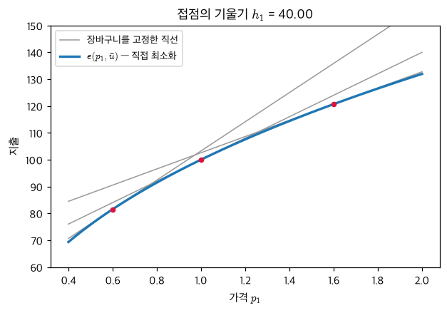

# 그림 2 — 재최적화 이득과 직접효과를 log-log 로 가른다
dps = np.logspace(-3, 0, 25)
gapcurve = np.array([(p1 + d) * h1n + p2 * h2n - emin(p1 + d, p2, ubar)[2] for d in dps])

fig, ax = plt.subplots(figsize=(6.4, 4.0))
ax.loglog(dps, h1n * dps, lw=1.6, color='seagreen',
          label='직접효과 $h_1\\Delta p_1$ (기울기 1)')
ax.loglog(dps, gapcurve, lw=2.2, color='C0',
          label="재최적화 이득 $p'\\cdot h(p)-e(p')$ (기울기 2)")
ax.loglog(dps, coef * dps ** 2, ':', color='k', lw=1.2,
          label='2차항 $%.0f\\,(\\Delta p_1)^2$' % coef)
for d in (0.01, 0.1, 0.5):
    ax.plot([d], [gaps[d]], 'o', color='crimson', ms=5, zorder=5)
pow10 = FuncFormatter(lambda v, _: '$10^{%d}$' % int(round(np.log10(v))))
for axis in (ax.xaxis, ax.yaxis):      # 눈금을 10의 거듭제곱으로 직접 적는다
    axis.set_major_locator(LogLocator(base=10.0))
    axis.set_major_formatter(pow10)
    axis.set_minor_formatter(NullFormatter())
ax.set_xlabel('가격 변화 $\\Delta p_1$')
ax.set_ylabel('크기')
ax.legend(fontsize=8, loc='upper left')
ax.set_title('국소 기울기 %.2f (0.01-0.1) → %.2f (0.1-0.5)' % (s_small, s_large))
plt.show()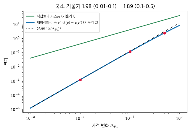

# 예측 항목 셋에 대응하는 수치를 한자리에 모은다
print('%-4s %-46s %s' % ('항목', '계산값', '예측값'))
print('%-4s %-46s %s' % ('1',
      'de/dp1 = %.5f, h1 = %.5f, 상대오차 %.1e' % (de_dp1, h1n, rel1), 'h1 = 40.0, 1e-5 이내'))
print('%-4s %-46s %s' % ('2',
      '차 %.4f / %.3f / %.3f' % (gaps[0.01], gaps[0.1], gaps[0.5]), '0.0012 / 0.114 / 2.39'))
print('%-4s %-46s %s' % ('',
      '기울기 %.2f (0.01-0.1) / %.2f (0.1-0.5)' % (s_small, s_large), '1.98 / 1.89'))
print('%-4s %-46s %s' % ('3',
      'dv/dw = %.4f, lambda* = %.4f' % (dv_dw, lam), '0.3366'))
print('%-4s %-46s %s' % ('',
      'Roy = %.4f, x1* = %.4f' % (roy, x1s), '40.0'))